5.1: Two-level Systems

The discussion of the bra-ket formalism in the previous chapter was peppered with numerous illustrations of its main concepts on the example of "spins- \(1 / 2\) " - systems with the smallest non-trivial (two-dimensional) Hilbert space, in which the bra- and ket-vectors of an arbitrary quantum state \(\alpha\) may be represented as a linear superposition of just two basis vectors, for example \[|\alpha\rangle=\alpha_{\uparrow}|\uparrow\rangle+\alpha_{\downarrow}|\downarrow\rangle,\] where the states \(\uparrow\) and \(\downarrow\) were defined as the eigenstates of the Pauli matrix \(\sigma_{z}-\) see Eq. (4.105). For the genuine spin- \(-\frac{2}{2}\) particles, such as electrons, placed in a \(z\)-oriented time-independent magnetic field, these states are the stationary "spin-up" and "spin-down" stationary states of the Pauli Hamiltonian (4.163), with the corresponding two energy levels (4.167). However, an approximate but reasonable quantum description of some other important systems may also be given in such Hilbert space.

For example, as was discussed in Sec. 2.6, two weakly coupled space-localized orbital states of a spin-free particle are sufficient for an approximate description of its quantum oscillations between two potential wells. A similar coupling of two traveling waves explains the energy band splitting in the weak-potential approximation of the band theory - Sec. 2.7. As will be shown in the next chapter, in systems with time-independent Hamiltonians, such situation almost unavoidably appears each time when two energy levels are much closer to each other than to other levels. Moreover, as will be shown in Sec. 6.5, a similar truncated description is adequate even in cases when two levels \(E_{n}\) and \(E_{n}\) ’ of an unperturbed system are not close to each other, but the corresponding states become coupled by an applied ac field of a frequency \(\omega\) very close to the difference \(\left(E_{n}-E_{n}^{\prime}\right) / \hbar .\) Such two-level systems (alternatively called "spin- \(1 / 2\)-like" systems) are nowadays the focus of additional attention in the view of prospects of their use for quantum information processing and encryption.

First, the most general form of the Hamiltonian of a two-level system is represented, in an arbitrary basis, by a \(2 \times 2\) matrix \[\mathrm{H}=\left(\begin{array}{ll} H_{11} & H_{12} \\ H_{21} & H_{22} \end{array}\right)\] According to the discussion in Secs. 4.3-4.5, since the Hamiltonian operator has to be Hermitian, the diagonal elements of the matrix \(\mathrm{H}\) have to be real, and its off-diagonal elements be complex conjugates

\({ }^{1}\) In the last context, to be discussed in Sec. \(8.5\), the two-level systems are usually called qubits. of each other: \(H_{21}=H_{12}\). As a result, we may not only represent \(H\) as a linear combination (4.106) of the identity matrix and the Pauli matrices but also reduce it to a more specific form: \[\mathrm{H}=b \mathrm{I}+\mathbf{c} \cdot \boldsymbol{\sigma}=\left(\begin{array}{cc} b+c_{z} & c_{x}-i c_{y} \\ c_{x}+i c_{y} & b-c_{z} \end{array}\right) \equiv\left(\begin{array}{cc} b+c_{z} & c_{-} \\ c_{+} & b-c_{z} \end{array}\right), \quad c_{\pm} \equiv c_{x} \pm i c_{y},\] where the scalar \(b\) and the Cartesian components of the vector \(\mathbf{c}\) are real \(c\)-number coefficients: \[b=\frac{H_{11}+H_{22}}{2}, \quad c_{x}=\frac{H_{12}+H_{21}}{2} \equiv \operatorname{Re} H_{21}, \quad c_{y}=\frac{H_{21}-H_{12}}{2 i} \equiv \operatorname{Im} H_{21}, \quad c_{z}=\frac{H_{11}-H_{22}}{2} .\] If such Hamiltonian does not depend on time, the corresponding characteristic equation (4.103) for the system’s energy levels \(E_{\pm}\), \[\left|\begin{array}{cc} b+c_{z}-E & c_{-} \\ c_{+} & b-c_{z}-E \end{array}\right|=0,\] is a simple quadratic equation, with the following solutions: \[E_{\pm}=b \pm c \equiv b \pm\left(c_{+} c_{-}+c_{z}^{2}\right)^{1 / 2} \equiv b \pm\left(c_{x}^{2}+c_{y}^{2}+c_{z}^{2}\right)^{1 / 2} \equiv \frac{H_{11}+H_{22}}{2} \pm\left[\left(\frac{H_{11}-H_{22}}{2}\right)^{2}+\left|H_{21}\right|^{2}\right]^{1 / 2} .\] The parameter \(b \equiv\left(H_{11}+H_{22}\right) / 2\) evidently gives the average energy \(E^{(0)}\) of the system, which does not contribute to the level splitting \[\Delta E \equiv E_{+}-E_{-}=2 c \equiv 2\left(c_{x}^{2}+c_{y}^{2}+c_{z}^{2}\right)^{1 / 2} \equiv\left[\left(H_{11}-H_{22}\right)^{2}+4\left|H_{21}\right|^{2}\right]^{1 / 2} .\] So, the splitting is a hyperbolic function of the coefficient \(c_{z} \equiv\left(H_{11}-H_{22}\right) / 2\). A plot of this function is the famous level-anticrossing diagram (Fig. 1), which has already been discussed in Sec. \(2.7\) in the particular context of the weak-potential limit of the 1D band theory.

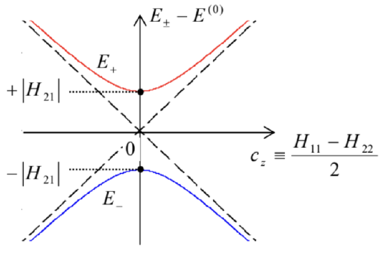Fig. 5.1. The level-anticrossing diagram for an arbitrary two-level system.

The physics of the diagram becomes especially clear if the two states of the basis used to spell out the matrix (2), may be interpreted as the stationary states of two potentially independent subsystems, with the energies, respectively, \(H_{11}\) and \(H_{22}\). (For example, in the case of two weakly coupled potential wells discussed in Sec. 2.6, these are the ground-state energies of two distant wells.) Then the offdiagonal elements \(c_{-} \equiv H_{12}\) and \(c_{+} \equiv H_{21}=H_{12}{ }^{*}\) describe the subsystem coupling, and the level anticrossing diagram shows how do the eigenenergies of the coupled system depend (at fixed coupling) on the difference of the subsystem energies. As was already discussed in Sec. 2.7, the most striking feature of the diagram is that any non-zero coupling \(\left|c_{\pm}\right| \equiv\left(c_{x}{ }^{2}+c_{y}{ }^{2}\right)^{1 / 2}\) changes the topology of the eigenstate energies, creating a gap of the width \(\Delta E\).

As it follows from our discussions of particular two-level systems in Secs. \(2.6\) and 4.6, their dynamics also has a general feature - the quantum oscillations. Namely, if we put any two-level system into any initial state different from one of its eigenstates \(\pm\), and then let it evolve on its own, the probability of its finding the system in any of the "partial" states exhibits oscillations with the frequency \[\Omega=\frac{\Delta E}{\hbar} \equiv \frac{E_{+}-E_{-}}{\hbar}=2 c,\] lowest at the exact subsystem symmetry \(\left(c_{z}=0\right.\), i.e. \(\left.H_{11}=H_{22}\right)\), when it is proportional to the coupling strength: \(\Omega_{\min }=2\left|c_{\pm}\right| / \hbar \equiv 2\left|H_{12}\right| / \hbar=2\left|H_{21}\right| / \hbar\).

In the case discussed in Sec. 2.6, these are the oscillations of a particle between the two coupled potential wells (or rather of the probabilities to find it in either well) - see, e.g., Eqs. (2.181). On the other hand, for a spin- \(1 / 2\) particle in an external magnetic field, these oscillations take the form of spin precession in the plane normal to the field, with periodic oscillations of its Cartesian components (or rather their expectation values) - see, e.g., Eqs. (4.173)-(4.174). Some other examples of the quantum oscillations in two-level systems may be rather unexpected; for example, the ammonium molecule \(\mathrm{NH}_{3}\) (Fig. 2) has two symmetric states that differ by the inversion of the nitrogen atom relative to the plane of the three hydrogen atoms, which are weakly coupled due to quantum-mechanical tunneling of the nitrogen atom through the plane of the hydrogen atoms. \({ }^{2}\) Since for this particular molecule, in the absence of external fields, the level splitting \(\Delta E\) corresponds to an experimentally convenient frequency \(\Omega / 2 \pi \approx 24 \mathrm{GHz}\), it played an important historic role at the initial development of the atomic frequency standards and microwave quantum generators (masers) in the early \(1950 \mathrm{~s},{ }^{3}\) which paved the way toward laser technology.

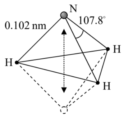Fig. 5.2. An ammonia molecule and its inversion.

Now let us now discuss a very convenient geometric representation of an arbitrary state \(\alpha\) of (any!) two-level system. As Eq. (1) shows, such state is completely described by two complex coefficients ( \(c\)-numbers) - say, \(\alpha \uparrow\) and \(\alpha \downarrow\). If the vectors of the basis states \(\uparrow\) and \(\downarrow\) are normalized, then these coefficients must obey the following restriction: \[W_{\Sigma}=\langle\alpha \mid \alpha\rangle=\left(\left\langle\uparrow\left|\alpha_{\uparrow}^{*}+\langle\downarrow| \alpha_{\downarrow}^{*}\right)\left(\alpha_{\uparrow}|\uparrow\rangle+\alpha_{\downarrow}|\downarrow\rangle\right)=\alpha_{\uparrow}^{*} \alpha_{\uparrow}+\alpha_{\downarrow}^{*} \alpha_{\downarrow}=\left|\alpha_{\uparrow}\right|^{2}+\left|\alpha_{\downarrow}\right|^{2}=1 .\right.\right.\] This requirement is automatically satisfied if we take the moduli of \(\alpha \uparrow\) and \(\alpha \downarrow\) equal to the sine and cosine of the same (real) angle. Thus we may write, for example, \[\alpha_{\uparrow}=\cos \frac{\theta}{2} e^{i \gamma}, \quad \alpha_{\downarrow}=\sin \frac{\theta}{2} e^{i(\gamma+\varphi)} .\] Moreover, according to the general Eq. (4.125), if we deal with just one system, \({ }^{4}\) the common phase factor \(\exp \{i \gamma\}\) drops out of the calculation of any expectation value, so that we may take \(\gamma=0\), and Eq. (10) is reduced to \[\alpha_{\uparrow}=\cos \frac{\theta}{2}, \quad \alpha_{\downarrow}=\sin \frac{\theta}{2} e^{i \varphi} .\] The reason why the argument of these sine and cosine functions is usually taken in the form \(\theta / 2\), becomes clear from Fig. 3a: Eq. (11) conveniently maps each state \(\alpha\) of a two-level system on a certain representation point on a unit-radius Bloch sphere, \({ }^{5}\) with the polar angle \(\theta\) and the azimuthal angle \(\varphi\).

Fig. 5.3. The Bloch sphere: (a) the representation of an arbitrary state (solid red point) and the eigenstates of the Pauli matrices (dotted points), and (b, c) the two-level system’s evolution: (b) in a constant "field" \(c\) directed along the \(z\)-axis, and (c) in a field of arbitrary orientation.

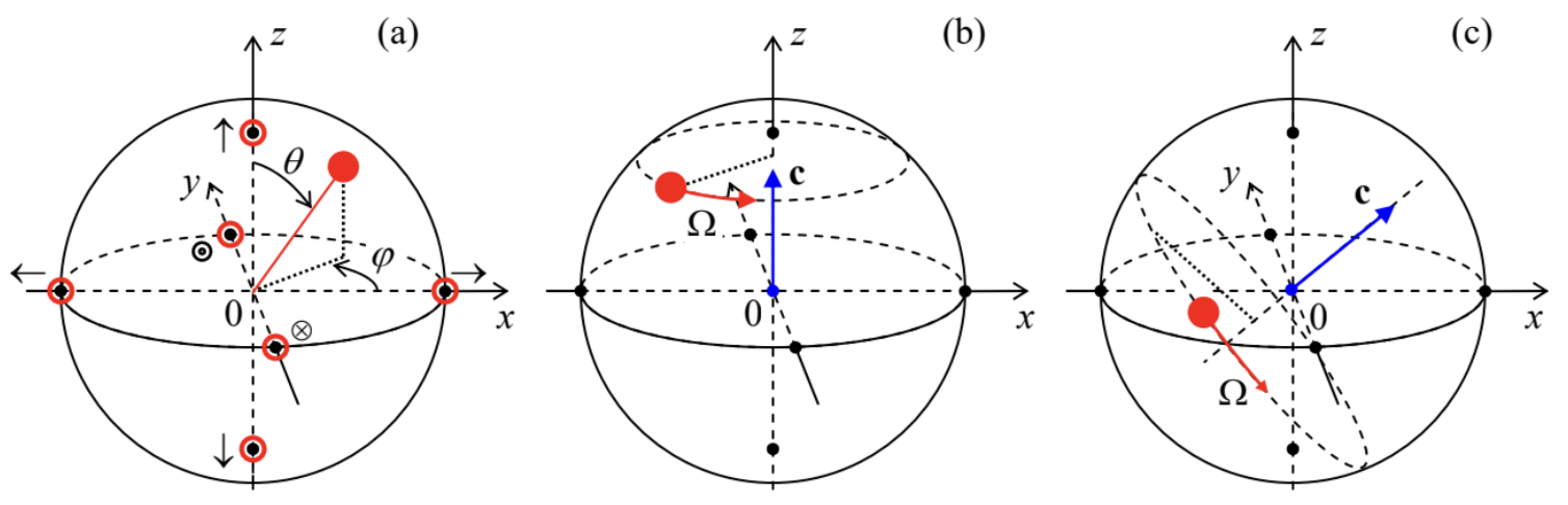
In particular, the basis state \(\uparrow\), described by Eq. (1) with \(\alpha \uparrow=1\) and \(\alpha \downarrow=0\), corresponds to the North Pole of the sphere \((\theta=0)\), while the opposite state \(\downarrow\), with \(\alpha \uparrow=0\) and \(\alpha_{\downarrow}=1\), to its South Pole ( \(\theta\) \(=\pi\) ). Similarly, the eigenstates \(\rightarrow\) and \(\leftarrow\) of the matrix \(\sigma_{x}\), described by Eqs. (4.122), i.e. having \(\alpha \uparrow=\) \(1 / \sqrt{2}\) and \(\alpha_{\downarrow}=\pm 1 / \sqrt{2}\), correspond to the equator \((\theta=\pi / 2)\) points with, respectively, \(\varphi=0\) and \(\varphi=\pi\). Two more special points (denoted in Fig. 3a as \(\odot\) and \(\otimes\) ) are also located on the sphere’s equator, at \(\theta=\) \(\pi / 2\) and \(\varphi=\pm \pi / 2\); it is easy to check that they correspond to the eigenstates of the matrix \(\sigma_{y}\) (in the same \(z\)-basis).

To understand why such mutually perpendicular location of these three special point pairs on the Bloch sphere is not occasional, let us plug Eqs. (11) into Eqs. (4.131)-(4.133) for the expectation values of the spin- \(-\frac{1}{2}\) components. In terms of the Pauli vector operator \((4.117), \sigma \equiv \mathbf{S} /(\hbar / 2)\), the result is \[\left\langle\sigma_{x}\right\rangle=\sin \theta \cos \varphi, \quad\left\langle\sigma_{y}\right\rangle=\sin \theta \sin \varphi, \quad\left\langle\sigma_{z}\right\rangle=\cos \theta,\] showing that the radius vector of any representation point is just the expectation value of \(\sigma\).

Now let us use Eq. (3) to see how does the representation point moves in various cases, ignoring the term \(b\) I - which, again, describes the offset of the total energy of the system relative to some reference level, and does not affect its dynamics. First of all, according to Eq. (4.158), in the case \(\mathbf{c}=0\) (when the Hamiltonian operator turns to zero, and hence the state vectors do not depend on time) the point does not move at all, and its position is determined by initial conditions, i.e. by the system’s preparation. If \(\mathbf{c} \neq 0\), we may re-use some results of Sec. 4.6, obtained for the Pauli Hamiltonian (4.163a), which coincides with Eq. (3) if \(^{6}\) \[\mathbf{c}=-\gamma \mathscr{B} \frac{\hbar}{2}\] In particular, if the field \(\mathscr{R}\), and hence the vector \(\mathbf{c}\), is directed along the \(z\)-axis and is time-independent, Eqs. (4.170) and (4.173)-(4.174) show that the representation point \(\langle\sigma\rangle\) on the Bloch sphere rotates within a plane normal to this axis (see Fig. 3b) with the angular velocity \[\frac{d \varphi}{d t} \equiv \Omega=-\gamma \mathscr{B}_{z} \equiv \frac{2 c_{z}}{\hbar} .\] Almost evidently, since the selection of the coordinate axes is arbitrary, this picture should remain valid for any orientation of the vector \(\mathbf{c}\), with the representation point rotating, on the Bloch sphere, around it direction, with the angular speed \(|\Omega|=2 c / \hbar-\) see Fig. \(3 \mathrm{c}\). This fact may be proved using any picture of the quantum dynamics, discussed in Sec. 4.6. Actually, the reader may already have done that by solving Problems \(4.25\) and \(4.26\), just to see that even for the particular, simple initial state of the system ( \(\uparrow\) ), the final results for the Cartesian components of the vector \(\langle\boldsymbol{\sigma}\rangle\) are somewhat bulky. However, this description may be readily simplified, even for arbitrary time dependence of the "field" vector \(\mathbf{c}(t)\) in Eq. (3), using the (geometric) vector language.

Indeed, let us rewrite Eq. (3) (again, with \(b=0\) ) in the operator form, \[\hat{H}=\mathbf{c}(t) \cdot \hat{\boldsymbol{\sigma}},\] valid in an arbitrary basis. According to Eq. (4.199), the corresponding Heisenberg equation of motion for the \(j^{\text {th }}\) Cartesian components of the vector-operator \(\hat{\boldsymbol{\sigma}}\) (which does not depend on time explicitly, so that \(\partial \hat{\sigma} / \partial t=0\) ) is

\[i \hbar \dot{\hat{\sigma}}_{j}=\left[\hat{\sigma}_{j}, \hat{H}\right] \equiv\left[\hat{\sigma}_{j}, \mathbf{c}(t) \cdot \hat{\boldsymbol{\sigma}}\right] \equiv\left[\hat{\sigma}_{j}, \sum_{j^{\prime}=1}^{3} c_{j^{\prime}}(t) \hat{\sigma}_{j^{\prime}}\right] \equiv \sum_{j^{\prime}=1}^{3} c_{j^{\prime}}(t)\left[\hat{\sigma}_{j}, \hat{\sigma}_{j^{\prime}}\right] .\] Now using the commutation relations (4.155), which remain valid in any basis and in any picture of time evolution, \({ }^{7}\) we get \[i \hbar \dot{\hat{\sigma}}_{j}=2 i \sum_{j^{\prime}=1}^{3} c_{j^{\prime}}(t) \hat{\sigma}_{j^{\prime \prime}} \varepsilon_{j j j^{\prime \prime}},\] where \(j\) ’, is the index, or the same set \(\{1,2,3\}\), complementary to \(j\) and \(j\) ’ \(\left(j^{\prime \prime} \neq j, j^{\prime}\right)\), and \(\varepsilon_{j j^{\prime} j^{\prime \prime}}\) is the Levi-Civita symbol. \({ }^{8}\) But it is straightforward to verify that the usual vector product of two \(3 \mathrm{D}\) vectors may be represented in a similar Cartesian-component form: \[(\mathbf{a} \times \mathbf{b})_{j}=\left|\begin{array}{lll} \mathbf{n}_{1} & \mathbf{n}_{2} & \mathbf{n}_{3} \\ a_{1} & a_{2} & a_{3} \\ b_{1} & b_{2} & b_{3} \end{array}\right|_{j}=\sum_{j^{\prime}=1}^{3} a_{j^{\prime}} b_{j^{\prime}} \varepsilon_{j j j^{\prime \prime}},\] As a result, Eq. (17) may be rewritten in a vector form - or rather several equivalent forms: \[i \hbar \dot{\hat{\sigma}}_{j}=2 i[\mathbf{c}(t) \times \hat{\boldsymbol{\sigma}}]_{j}, \quad \text { i.e. } i \hbar \dot{\hat{\boldsymbol{\sigma}}}=2 i \mathbf{c}(t) \times \hat{\boldsymbol{\sigma}}, \quad \text { or } \dot{\hat{\boldsymbol{\sigma}}}=\frac{2}{\hbar} \mathbf{c}(t) \times \hat{\boldsymbol{\sigma}}, \quad \text { or } \dot{\hat{\boldsymbol{\sigma}}}=\boldsymbol{\Omega}(t) \times \hat{\boldsymbol{\sigma}},\] where the vector \(\Omega\) is defined as \[\hbar \boldsymbol{\Omega}(t) \equiv 2 \mathbf{c}(t)\]

• an evident generalization of Eq. (14). \({ }^{9}\) As we have seen in Sec. 4.6, any linear relation between two Heisenberg operators is also valid for the expectation values of the corresponding observables, so that the last form of Eq. (19) yields:

\[\langle\dot{\boldsymbol{\sigma}}\rangle=\boldsymbol{\Omega}(t) \times\langle\boldsymbol{\sigma}\rangle .\] But this is the well-known kinematic formula \({ }^{10}\) for the rotation of a constant-length classical 3D vector \(\langle\boldsymbol{\sigma}\rangle\) around the instantaneous direction of the vector \(\boldsymbol{\Omega}(t)\), with the instantaneous angular velocity \(\Omega(t)\). So, the time evolution of the representation point on the Bloch sphere is quite simple, especially in the case of a time-independent \(\mathbf{c}\), and hence \(\Omega\) - see Fig. 3c. \({ }^{11}\) Note that it is sufficient to turn off the field to stop the precession instantly. (Since Eq. (21) is the first-order differential equation, the representation point has no effective inertia. \({ }^{12}\) ) Hence, changing the direction and the magnitude of the effective external field, it is possible to drive the representation point of a two-level system from any initial position to any final position on the Bloch sphere, i.e. make the system take any of its possible quantum states.

In the particular case of a spin- \(1 / 2\) in a magnetic field \(\mathscr{B}(t)\), it is more customary to use Eqs. (13) and \((20)\) to rewrite Eq. (21) as the following equation for the expectation value of the spin vector \(\mathbf{S}=\) ( \(\hbar / 2\) ) \(\sigma\) : \[\langle\dot{\mathbf{S}}\rangle \equiv \gamma\langle\mathbf{S}\rangle \times \mathscr{B}(t)\] As we know from the discussion in Chapter 4, such a classical description of the spin’s evolution does not give a full picture of the quantum reality; in particular, it does not describe the possible large uncertainties of its components - see, e.g., Eqs. (4.135). The situation, however, is different for a collection of \(N \gg 1\) similar, non-interacting spins, initially prepared to be in the same state - for example by polarizing all spins with a strong external field \(\mathscr{R}_{0}\), at relatively low temperatures \(T\), with \(k_{\mathrm{B}} T<\gamma \mathscr{B}_{0} \hbar\). (A practically important example of such a collection is a set of nuclear spins in macroscopic condensed-matter samples, where the spin interaction with each other and the environment is typically very small.) For such a collection, Eq. (22) is still valid, while the relative uncertainty of the resulting sample’s magnetization \(\mathbf{M}=n\langle\mathbf{m}\rangle=n \gamma\langle\mathbf{S}\rangle\) (where \(n \equiv N / V\) is the spin density) is proportional to \(1 / N^{1 / 2}<<1\). Thus, the evolution of magnetization may be described, with good precision, by the essentially classical equation (valid for any spin, not necessarily spin- \(1 / 2\) ): \[\dot{\mathbf{M}}=\gamma \mathbf{M} \times \mathscr{R}(t) .\] This equation, or the equivalent set of three Bloch equations 13 for its Cartesian components, with the right-hand side augmented with small terms describing the effects of dephasing and relaxation (to be discussed in Chapter 7), is used, in particular, to describe the magnetic resonance, taking place when the frequency (4.164) of the spin’s precession in a strong do magnetic field approaches the frequency of an additionally applied (and usually weak) ac field. \({ }^{14}\)

---

\({ }^{1}\) This is why let me spend a bit more time reviewing the main properties of an arbitrary two-level system.

\({ }^{2}\) Since the hydrogen atoms are much lighter, it would be fairer to speak about the tunneling of their triangle around the (nearly immobile) nitrogen atom.

\({ }^{3}\) In particular, these molecules were used in the demonstration of the first maser by C. Townes’ group in \(1954 .\)

\({ }^{4}\) If you need a reminder of why this condition is crucial, please revisit the discussion at the end of Sec. 1.6. Note also that the mutual phase shifts between different qubits are important, in particular, for quantum information processing (see Sec. \(8.5\) below), so that most discussions of these applications have to start from Eq. (10) rather than Eq. (11).

\({ }^{5}\) This representation was suggested in 1946 by the same Felix Bloch who has pioneered the energy band theory discussed in Chapters 2-3.

\({ }^{6}\) This correspondence justifies using the use of term "field" for the vector \(\mathbf{c}\).

\({ }^{7}\) Indeed, if some three operators in the Schrödinger picture are related as \(\left[\hat{A}_{\mathrm{s}}, \hat{B}_{\mathrm{S}}\right]=\hat{C}_{\mathrm{S}}\), then according to Eq. (4.190), in the Heisenberg picture: \[\left[\hat{A}_{\mathrm{H}}, \hat{B}_{\mathrm{H}}\right]=\left[\hat{u}^{\dagger} \hat{A}_{\mathrm{H}} \hat{u}, \hat{u}^{\dagger} \hat{B}_{\mathrm{H}} \hat{u}\right] \equiv \hat{u}^{\dagger} \hat{A}_{\mathrm{H}} \hat{u} \hat{u}^{\dagger} \hat{B}_{\mathrm{H}} \hat{u}-\hat{u}^{\dagger} \hat{B}_{\mathrm{H}} \hat{u} \hat{u}^{\dagger} \hat{A}_{\mathrm{H}} \hat{u} \equiv \hat{u}^{\dagger}\left[\hat{A}_{\mathrm{s}}, \hat{B}_{\mathrm{S}}\right] \hat{u} \equiv \hat{u}^{\dagger} \hat{C}_{\mathrm{S}} \hat{u}=\hat{C}_{\mathrm{H}} .\] \({ }^{8}\) See, e.g., MA Eq. (9.2). Note that in Eqs. (17)-(18) and similar expressions below, the condition \(j^{\prime \prime} \neq j, j^{\prime}\) may be (and frequently is) replaced by the summation over not only \(j\) ’, but also \(j\) ", in their right-hand sides.

\({ }^{9}\) It is also easy to verify that in the particular case \(\Omega=\Omega \mathbf{n}_{z}\), Eqs. (19) are reduced, in the \(z\)-basis, to Eqs. (4.200) for the spin-1/2 vector matrix \(\mathbf{S}=(\hbar / 2) \sigma\).

\({ }^{10}\) See, e.g., CM Sec. 4.1, in particular Eq. (4.8).

\({ }^{11}\) The bulkiness of the solutions of Problems \(4.25\) and \(4.26\) (which were offered just as useful exercises in quantum dynamic formalisms) reflects the awkward expression of the resulting circular motion of the vector \(\langle\boldsymbol{\sigma}\rangle\) (see Fig. 3c) via its Cartesian components.

\({ }^{12}\) This is also true for the classical angular momentum \(\mathbf{L}\) at its torque-induced precession - see, e.g., \(\mathrm{CM}\) Sec. \(4.5\).

\({ }^{13}\) They were introduced by F. Bloch in the same 1946 paper as the Bloch-sphere representation.

\({ }^{14}\) The quantum theory of this effect will be discussed in the next chapter.