5.6: Revisiting Spherically-symmetric Problems

One more blank spot to fill has been left by our study, in Sec. 3.6, of wave mechanics of particle motion in spherically-symmetric 3D potentials. Indeed, while the azimuthal components of the eigenfunctions (the spherical harmonics) of such systems are very simple, \[\psi_{m}=(2 \pi)^{-1 / 2} e^{i m \varphi}, \text { with } m=0, \pm 1, \pm 2, \ldots,\] their polar components include the associated Legendre functions \(P_{l}^{m}(\cos \theta)\), which may be expressed via elementary functions only indirectly - see Eqs. (3.165) and (3.168). This makes all the calculations less than transparent and, in particular, does not allow a clear insight into the origin of the very simple energy spectrum of such systems - see, e.g., Eq. (3.163). The bra-ket formalism, applied to the angular momentum operator, not only enables such insight and produces a very convenient tool for many calculations involving spherically-symmetric potentials, but also opens a clear way toward the unification of the orbital momentum with the particle’s spin - the latter task to be addressed in the next section.

Let us start by using the correspondence principle to spell out the quantum-mechanical vector operator of the orbital angular momentum \(\mathbf{L} \equiv \mathbf{r} \times \mathbf{p}\) of a point particle: \[\hat{\mathbf{L}} \equiv \hat{\mathbf{r}} \times \hat{\mathbf{p}}=\left|\begin{array}{ccc} \mathbf{n}_{x} & \mathbf{n}_{y} & \mathbf{n}_{z} \\ \hat{r}_{1} & \hat{r}_{2} & \hat{r}_{3} \\ \hat{p}_{1} & \hat{p}_{2} & \hat{p}_{3} \end{array}\right|, \quad \text { i.e. } \hat{L}_{j} \equiv \sum_{j^{\prime}=1}^{3} \hat{r}_{j^{\prime}} \hat{p}_{j^{\prime}} \varepsilon_{j j^{\prime \prime} \prime^{\prime \prime}},\] where each of the indices \(j, j^{\prime}\), and \(j\) ’" may take values 1,2 , and 3 (with \(j\) ’ \(\neq j, j\) ’), and \(\varepsilon_{j j \prime}\) ", is the LeviCivita permutation symbol, which we have already used in Sec. 4.5, and also in Sec. 1 of this chapter, in similar expressions (17)-(18). From this definition, we can readily calculate the commutation relations for all Cartesian components of operators \(\hat{\mathbf{L}}, \hat{\mathbf{r}}\), and \(\hat{\mathbf{p}}\); for example, \[\left[\hat{L}_{j}, \hat{r}_{j^{\prime}}\right]=\left[\sum_{k=1}^{3} \hat{r}_{k} \hat{p}_{j^{\prime \prime}} \varepsilon_{j k j^{\prime \prime}}, \hat{r}_{j^{\prime}}\right] \equiv-\sum_{k=1}^{3} \hat{r}_{k}\left[\hat{r}_{j^{\prime}}, \hat{p}_{j^{\prime \prime}}\right] \varepsilon_{j k j^{\prime \prime}}=-i \hbar \sum_{k=1}^{3} \hat{r}_{k} \delta_{j j^{\prime \prime}} \varepsilon_{j k j^{\prime \prime}} \equiv i \hbar \sum_{k=1}^{3} \hat{r}_{k} \varepsilon_{j j^{\prime} k} \equiv i \hbar \hat{r}_{j^{\prime \prime}} \varepsilon_{j j j^{\prime \prime}},\] The summary of all these calculations may be represented in similar compact forms: \[\left[\hat{L}_{j}, \hat{r}_{j^{\prime}}\right]=i \hbar \hat{r}_{j^{\prime \prime}} \varepsilon_{j j j^{\prime \prime}}, \quad\left[\hat{L}_{j}, \hat{p}_{j^{\prime}}\right]=i \hbar \hat{p}_{j^{\prime \prime}} \varepsilon_{j j^{\prime \prime}}, \quad\left[\hat{L}_{j}, \hat{L}_{j^{\prime}}\right]=i \hbar \hat{L}_{j^{\prime \prime}} \varepsilon_{j j j^{\prime \prime}} ;\] the last of them shows that the commutator of two different Cartesian components of the vector-operator \(\hat{\mathbf{L}}\) is proportional to its complementary component.

Also introducing, in a natural way, the (scalar!) operator of the observable \(L^{2} \equiv|\mathbf{L}|^{2}\), \[\hat{L}^{2} \equiv \hat{L}_{x}^{2}+\hat{L}_{y}^{2}+\hat{L}_{z}^{2} \equiv \sum_{j=1}^{3} L_{j}^{2},\] it is straightforward to check that this operator commutes with each of the Cartesian components: \[\left[\hat{L}^{2}, \hat{L}_{j}\right]=0\] This result, at the first sight, may seem to contradict the last of Eqs. (149). Indeed, haven’t we learned in Sec. \(4.5\) that commuting operators (e.g., \(\hat{L}^{2}\) and any of \(\hat{L}_{j}\) ) share their eigenstate sets? If yes, shouldn’t this set has to be common for all four angular momentum operators? The resolution in this paradox may be found in the condition that was mentioned just after Eq. (4.138), but (sorry!) was not sufficiently emphasized there. According to that relation, if an operator has degenerate eigenstates (i.e. if some \(A_{j}=\) \(A_{j}\) ’ even for \(j \neq j^{\prime}\) ), they should not be necessarily all shared by another compatible operator.

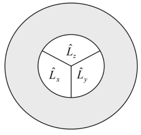
This is exactly the situation with the orbital angular momentum operators, which may be schematically shown on a Venn diagram (Fig. 10):45 the eigenstates of the operator \(\hat{L}^{2}\) are highly degenerate \({ }^{46}\) and their set is broader than those of any component operator \(\hat{L}_{j}\) (that, as will be shown below, are non-degenerate - until we consider particle’s spin).

Fig. 5.10. The Venn diagram showing the partitioning of the set of eigenstates of the operator \(\hat{L}^{2}\). Each inner sector corresponds to the states shared with one of the Cartesian component operators \(\hat{L}_{j}\), while the outer (shaded) ring represents the eigenstates of \(\hat{L}^{2}\) that are not shared with either of \(\hat{L}_{j}\) - for example, all linear combinations of the eigenstates of different component operators.

Let us focus on just one of these three joint sets of eigenstates - by tradition, of the operators \(\hat{L}^{2}\) and \(\hat{L}_{z}\). (This tradition stems from the canonical form of the spherical coordinates, in which the polar angle is measure from the \(z\)-axis. Indeed, in the coordinate representation we may write \[\hat{L}_{z} \equiv \hat{x} p_{y}-\hat{y} p_{x}=x\left(-i \hbar \frac{\partial}{\partial y}\right)-y\left(-i \hbar \frac{\partial}{\partial x}\right)=-i \hbar \frac{\partial}{\partial \varphi} .\] Writing the standard eigenproblem for the operator in this representation, \(\hat{L}_{z} \psi_{m}=L_{z} \psi_{m}\), we see that it is satisfied by the eigenfunctions (146), with eigenvalues \(L_{z}=\hbar m-\) which was already conjectured in Sec. 3.5.) More specifically, let us consider a set of eigenstates \(\{l, m\}\) corresponding to a certain degenerate eigenvalue of the operator \(\hat{L}^{2}\), and all possible eigenvalues of the operator \(\hat{L}_{z}\), i.e. all possible quantum numbers \(m\). (At this point, \(l\) is just some label of the eigenvalue of the operator \(\hat{L}^{2}\); it will be defined more explicitly in a minute.) To analyze this set, it is instrumental to introduce the socalled ladder (also called, respectively, "raising" and "lowering") operators \({ }^{47}\)

Ladder operators

\[\ \hat{L}_{\pm} \equiv \hat{L}_{x} \pm i \hat{L}_{y}.\]

It is simple (and hence left for the reader’s exercise) to use this definition and the last of Eqs. (149) to calculate the following commutators: \[\left[\hat{L}_{+}, \hat{L}_{-}\right]=2 \hbar \hat{L}_{z}, \quad \text { and }\left[\hat{L}_{z}, \hat{L}_{\pm}\right]=\pm \hbar \hat{L}_{\pm},\] and also to use Eqs. (149)-(150) to prove two other important operator relations: \[\hat{L}^{2}=\hat{L}_{z}^{2}+\hat{L}_{+} \hat{L}_{-}-\hbar \hat{L}_{z}, \quad \hat{L}^{2}=\hat{L}_{z}^{2}+\hat{L}_{-} \hat{L}_{+}+\hbar \hat{L}_{z} .\] Now let us rewrite the last of Eqs. (154) as \[\hat{L}_{z} \hat{L}_{\pm}=\hat{L}_{\pm} \hat{L}_{z} \pm \hbar \hat{L}_{\pm},\] and act by its both sides upon the ket-vector \(|l, m\rangle\) of an arbitrary common eigenstate: \[\hat{L}_{z} \hat{L}_{\pm}|l, m\rangle=\hat{L}_{\pm} \hat{L}_{z}|l, m\rangle \pm \hbar \hat{L}_{\pm}|l, m\rangle .\] Since the eigenvalues of the operator \(\hat{L}_{z}\) are equal to \(\hbar m\), in the first term of the right-hand side of Eq. (157) we may write \[\hat{L}_{z}|l, m\rangle=\hbar m|l, m\rangle .\] With that, Eq. (157) may be recast as \[\hat{L}_{z}\left(\hat{L}_{\pm}|l, m\rangle\right)=\hbar(m \pm 1)\left(\hat{L}_{\pm}|l, m\rangle\right) .\] In a spectacular similarity with Eqs. (78)-(79) for the harmonic oscillator, Eq. (159) means that the states \(\hat{L}_{\pm}|l, m\rangle\) are also eigenstates of the operator \(\hat{L}_{z}\), corresponding to eigenvalues \(\hbar(m \pm 1)\). Thus the ladder operators act exactly as the creation and annihilation operators of a harmonic oscillator, moving the system up or down a ladder of eigenstates - see Fig. 11 .

Fig. 5.11. The ladder diagram of the common eigenstates of the operators \(\hat{L}^{2}\) and \(\hat{L}_{z}\).

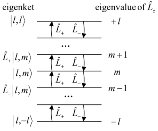
The most significant difference is that now the state ladder must end in both directions, because an infinite increase of \(|m|\), with whichever sign of \(m\), would cause the expectation values of the operator \[\hat{L}_{x}^{2}+\hat{L}_{y}^{2} \equiv \hat{L}^{2}-\hat{L}_{z}^{2},\] which corresponds to a non-negative observable, to become negative. Hence there have to be two states at both ends of the ladder, with such ket-vectors \(\left|l, m_{\max }\right\rangle\) and \(\left|l, m_{\min }\right\rangle\) that \[\hat{L}_{+}\left|l, m_{\max }\right\rangle=0, \quad \hat{L}_{-}\left|l, m_{\min }\right\rangle=0 .\] Due to the symmetry of the whole problem with respect to the replacement \(m \rightarrow-m\), we should have \(m_{\min }=-m_{\max }\). This \(m_{\max }\) is exactly the quantum number traditionally called \(l\), so that \[-l \leq m \leq+l .\] Evidently, this relation of quantum numbers \(m\) and \(l\) is semi-quantitatively compatible with the classical image of the angular momentum vector \(\mathbf{L}\), of the same length \(L\), pointing in various directions, thus affecting the value of its component \(L_{z}\). In this classical picture, however, \(L^{2}\) would be equal to the square of \(\left(L_{z}\right)_{\max }\), i.e. to \((\hbar l)^{2}\); however, in quantum mechanics, this is not so. Indeed, applying both parts of the second of the operator equalities (155) to the top state’s vector \(\left|l, m_{\max }\right\rangle \equiv|l, l\rangle\), we get \[\begin{aligned} \hat{L}^{2}|l, l\rangle &=\hbar \hat{L}_{z}|l, l\rangle+\hat{L}_{z}^{2}|l, l\rangle+\hat{L}_{-} \hat{L}_{+}|l, l\rangle=\hbar^{2} l|l, l\rangle+\hbar^{2} l^{2}|l, l\rangle+0 \\ & \equiv \hbar^{2} l(l+1)|l, l\rangle . \end{aligned}\] Since by our initial assumption, all eigenvectors \(|l, m\rangle\) correspond to the same eigenvalue of \(\hat{L}^{2}\), this result means that all these eigenvalues are equal to \(\hbar^{2} l(l+1)\). Just as in the case of the spin- \(1 / 2\) vector operators discussed in \(\mathrm{Sec} .4 .5\), the deviation of this result from \(\hbar^{2} l^{2}\) may be interpreted as the result of unavoidable uncertainties ("fluctuations") of the \(x\) - and \(y\)-components of the angular momentum, which give non-zero positive contributions to \(\left\langle L_{x}{ }^{2}\right\rangle\) and \(\left\langle L_{y}{ }^{2}\right\rangle\), and hence to \(\left\langle L^{2}\right\rangle\), even if the angular momentum vector is aligned with the \(z\)-axis in the best possible way.

(For various applications of the ladder operators (153), one more relation is convenient: \[\hat{L}_{\pm}|l, m\rangle=\hbar[l(l+1)-m(m \pm 1)]^{1 / 2}|l, m \pm 1\rangle .\] This equality, valid to the multiplier \(e^{i \varphi}\) with an arbitrary real phase \(\varphi\), may be readily proved from the above relations in the same way as the parallel Eqs. (89) for the harmonic-oscillator operators (65) were proved in Sec. 4; due to this similarity, the proof is also left for the reader’s exercise. \({ }^{48}\) )

Now let us compare our results with those of Sec. 3.6. Using the expression of Cartesian coordinates via the spherical ones exactly as this was done in Eq. (152), we get the following expressions for the ladder operators (153) in the coordinate representation:

Now plugging this relation, together with Eq. (152), into any of Eqs. (155), we get \[\hat{L}^{2}=-\hbar^{2}\left[\frac{1}{\sin \theta} \frac{\partial}{\partial \theta}\left(\sin \theta \frac{\partial}{\partial \theta}\right)+\frac{1}{\sin ^{2} \theta} \frac{\partial^{2}}{\partial \varphi^{2}}\right] .\] But this is exactly the operator (besides its division by the constant parameter \(2 m R^{2}\) ) that stands on the left-hand side of Eq. (3.156). Hence that equation, which was explored by the "brute-force" (wavemechanical) approach in Sec. 3.6, may be understood as the eigenproblem for the operator \(\hat{L}^{2}\) in the coordinate representation, with the eigenfunctions \(Y_{l}^{m}(\theta, \varphi)\) corresponding to the eigenkets \(|l, m\rangle\), and the eigenvalues \(L^{2}=2 m R^{2} E\). As a reminder, the main result of that, rather involved analysis was expressed by Eq. (3.163), which now may be rewritten as \[L_{l}^{2} \equiv 2 m R^{2} E_{l}=\hbar^{2} l(l+1),\] in full agreement with Eq. (163), which was obtained by much more efficient means based on the braket formalism. In particular, it is fascinating to see how easy it is to operate with the eigenvectors \(|l, m\rangle\), while the coordinate representations of these ket-vectors, the spherical harmonics \(Y_{l}^{m}(\theta, \varphi)\), may be only expressed by rather complicated functions - please have one more look at Eq. (3.171) and Fig. 3.20.

Note that all relations discussed in this section are not conditioned by any particular Hamiltonian of the system under analysis, though they (as well as those discussed in the next section) are especially important for particles moving in spherically-symmetric potentials.

---

\({ }^{45}\) This is just a particular example of the Venn diagrams (introduced in the 1880s by John Venn) that show possible relations (such as intersections, unions, complements, etc.) between various sets of objects, and are very useful tool in the general set theory.

\({ }^{46}\) Note that this particular result is consistent with the classical picture of the angular momentum vector: even when its length is fixed, the vector may be oriented in various directions, corresponding to different values of its Cartesian components. However, in the classical picture, all these components may be fixed simultaneously, while in the quantum picture this is not true.

\({ }^{47}\) Note a substantial similarity between this definition and Eqs. (65) for the creation/annihilation operators.

\({ }^{48}\) The reader is also challenged to use the commutation relations discussed above to prove one more important property of the common eigenstates of \(\hat{L}_{z}\) and \(\hat{L}^{2}\) : \[\left\langle l, m\left|\hat{r}_{j}\right| l^{\prime}, m^{\prime}\right\rangle=0, \quad \text { unless } l^{\prime}=l \pm 1 \text { and } m^{\prime}=\text { either } m \pm 1 \text { or } m \text {. }\] This property gives the selection rule for the orbital electric-dipole quantum transitions, to be discussed later in the course, especially in Sec. 9.3. (The final selection rules at these transitions may be affected by the particle’s spin - see the next section.)