5.4: Revisiting Harmonic Oscillator

Let us return to the 1D harmonic oscillator, now understood as any system, regardless of its physical nature, described by the Hamiltonian (4.237) with the potential energy (2.111): \[\hat{H}=\frac{\hat{p}^{2}}{2 m}+\frac{m \omega_{0}^{2} \hat{x}^{2}}{2} .\] In Sec. \(2.9\) we have used a "brute-force" (wave-mechanics) approach to analyze the eigenfunctions \(\psi_{n}(x)\) and eigenvalues \(E_{n}\) of this Hamiltonian, and found that, unfortunately, this approach required relatively complex mathematics, which does not enable an easy calculation of its key characteristics. Fortunately, the bra-ket formalism helps to make such calculations.

First, introducing normalized (dimensionless) operators of coordinates and momentum: 28 \[\hat{\xi} \equiv \frac{\hat{x}}{x_{0}}, \quad \hat{\zeta} \equiv \frac{\hat{p}}{m \omega_{0} x_{0}},\] where \(x_{0} \equiv\left(\hbar / m \omega_{0}\right)^{1 / 2}\) is the natural coordinate scale discussed in detail in Sec. \(2.9\), we can represent the Hamiltonian (62) in a very simple and \(x \leftrightarrow p\) symmetric form: \[\hat{H}=\frac{\hbar \omega_{0}}{2}\left(\hat{\xi}^{2}+\hat{\zeta}^{2}\right) .\] This symmetry, as well as our discussion of the very similar coordinate and momentum representations in Sec. 4.7, hints that much may be gained by treating the operators \(\hat{\xi}\) and \(\hat{\zeta}\) on equal footing. Inspired by this clue, let us introduce a new operator \[\hat{a} \equiv \frac{\hat{\xi}+i \hat{\zeta}}{\sqrt{2}} \equiv\left(\frac{m \omega_{0}}{2 \hbar}\right)^{1 / 2}\left(\hat{x}+i \frac{\hat{p}}{m \omega_{0}}\right)\] Since both operators \(\hat{\xi}\) and \(\hat{\zeta}\) correspond to real observables, i.e. have real eigenvalues and hence are Hermitian (self-adjoint), the Hermitian conjugate of the operator \(\hat{a}\) is simply its complex conjugate: \[\hat{a}^{\dagger} \equiv \frac{\hat{\xi}-i \hat{\zeta}}{\sqrt{2}} \equiv\left(\frac{m \omega_{0}}{2 \hbar}\right)^{1 / 2}\left(\hat{x}-i \frac{\hat{p}}{m \omega_{0}}\right)\] Because of the reason that will be clear very soon, \(\hat{a}^{\dagger}\) and \(\hat{a}\) (in this order!) are called the creation and annihilation operators.

Now solving the simple system of two linear equations (65) for \(\hat{\xi}\) and \(\hat{\zeta}\), we get the following reciprocal relations: \[\hat{\xi}=\frac{\hat{a}+\hat{a}^{\dagger}}{\sqrt{2}}, \quad \hat{\zeta}=\frac{\hat{a}-\hat{a}^{\dagger}}{\sqrt{2} i}, \quad \text { i.e. } \hat{x}=\left(\frac{\hbar}{m \omega_{0}}\right)^{1 / 2} \frac{\hat{a}+\hat{a}^{\dagger}}{\sqrt{2}}, \quad \hat{p}=\left(\hbar m \omega_{0}\right)^{1 / 2} \frac{\hat{a}-\hat{a}^{\dagger}}{\sqrt{2} i} \text {. }\] Our Hamiltonian (64) includes squares of these operators. Calculating them, we have to be careful to avoid swapping the new operators, because they do not commute. Indeed, for the normalized operators (63), Eq. (2.14) gives \[[\hat{\xi}, \hat{\zeta}] \equiv \frac{1}{x_{0}^{2} m \omega_{0}}[\hat{x}, \hat{p}]=i \hat{I},\] so that Eqs. (65) yield \[\begin{aligned} &\text { With such due caution, Eq. (66) gives } \\ &\qquad \hat{\xi}^{2}=\frac{1}{2}\left(\hat{a}^{2}+\hat{a}^{\dagger^{2}}+\hat{a} \hat{a}^{\dagger}+\hat{a}^{\dagger} \hat{a}\right), \quad \hat{\zeta}^{2}=-\frac{1}{2}\left(\hat{a}^{2}+\hat{a}^{\dagger^{2}}-\hat{a} \hat{a}^{\dagger}-\hat{a}^{\dagger} \hat{a}\right) . \end{aligned}\] Plugging these expressions back into Eq. (64), we get \[\hat{H}=\frac{\hbar \omega_{0}}{2}\left(\hat{a} \hat{a}^{\dagger}+\hat{a}^{\dagger} \hat{a}\right) .\] This expression is elegant enough, but may be recast into an even more convenient form. For that, let us rewrite the commutation relation (68) as \[\hat{a} \hat{a}^{\dagger}=\hat{a}^{\dagger} \hat{a}+\hat{I},\] and plug it into Eq. (70). The result is \[\hat{H}=\frac{\hbar \omega_{0}}{2}\left(2 \hat{a}^{\dagger} \hat{a}+\hat{I}\right) \equiv \hbar \omega_{0}\left(\hat{N}+\frac{1}{2} \hat{I}\right)\] where, in the last form, one more (evidently, Hermitian) operator, \[\hat{N} \equiv \hat{a}^{\dagger} \hat{a}\] has been introduced. Since, according to Eq. (72), the operators \(\hat{H}\) and \(\hat{N}\) differ only by the addition of the identity operator and multiplication by a \(c\)-number, these operators commute. Hence, according to the general arguments of Sec. 4.5, they share a set of stationary eigenstates \(n\) (they are frequently called the Fock states), and we can write the standard eigenproblem (4.68) for the new operator as \[\hat{N}|n\rangle=N_{n}|n\rangle,\] where \(N_{n}\) are some eigenvalues that, according to Eq. (72), determine also the energy spectrum of the oscillator: \[E_{n}=\hbar \omega_{0}\left(N_{n}+\frac{1}{2}\right) .\] So far, we know only that all eigenvalues \(N_{n}\) are real; to calculate them, let us carry out the following calculation - splendid in its simplicity and efficiency. Consider the result of the action of the operator \(\hat{N}\) on the ket-vector \(\hat{a}^{\dagger}|n\rangle\). Using the definition (73) and then the associative rule of the bra-ket formalism, we may write \[\hat{N}\left(\hat{a}^{\dagger}|n\rangle\right) \equiv\left(\hat{a}^{\dagger} \hat{a}\right)\left(\hat{a}^{\dagger}|n\rangle\right)=\hat{a}^{\dagger}\left(\hat{a} \hat{a}^{\dagger}\right)|n\rangle .\] Now using the commutation relation (71), and then Eq. (74), we may continue as \[\hat{a}^{\dagger}\left(\hat{a} \hat{a}^{\dagger}\right)|n\rangle=\hat{a}^{\dagger}\left(\hat{a}^{\dagger} \hat{a}+\hat{I}\right)|n\rangle=\hat{a}^{\dagger}(\hat{N}+\hat{I})|n\rangle=\hat{a}^{\dagger}\left(N_{n}+1\right)|n\rangle=\left(N_{n}+1\right)\left(\hat{a}^{\dagger}|n\rangle\right) .\] For clarity, let us summarize the result of this calculation: \[\hat{N}\left(\hat{a}^{\dagger}|n\rangle\right)=\left(N_{n}+1\right)\left(\hat{a}^{\dagger}|n\rangle\right) .\] Performing a similar calculation for the operator \(\hat{a}\), we get a similar formula: \[\hat{N}(\hat{a}|n\rangle)=\left(N_{n}-1\right)(\hat{a}|n\rangle) .\] It is time to stop calculations for a minute, and translate these results into plain English: if \(|n\rangle\) is an eigenket of the operator \(\hat{N}\) with the eigenvalue \(N_{n}\), then \(\hat{a}^{\dagger}|n\rangle\) and \(\hat{a}|n\rangle\) are also eigenkets of that operator, with the eigenvalues \(\left(N_{n}+1\right)\), and \(\left(N_{n}-1\right)\), respectively. This statement may be vividly represented on the so-called ladder diagram shown in Fig. 7.

Fig. 5.7. The "ladder diagram" of eigenstates of a \(1 \mathrm{D}\) harmonic oscillator. Arrows show the actions of the creation and annihilation operators on the eigenstates.

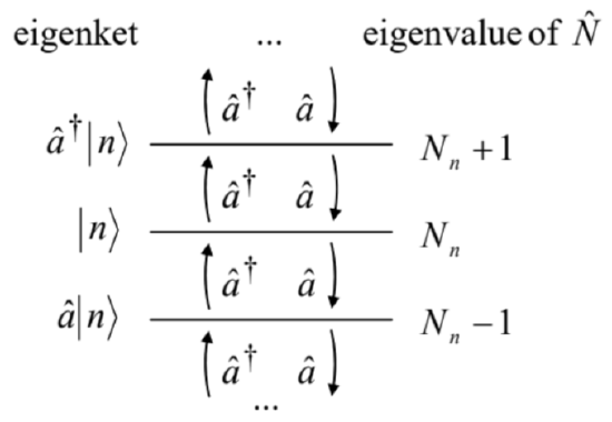
The operator \(\hat{a}^{\dagger}\) moves the system one step up this ladder, while the operator \(\hat{a}\) brings it one step down. In other words, the former operator creates a new excitation of the system, \({ }^{29}\) while the latter operator kills ("annihilates") such excitation. \({ }^{30}\) On the other hand, according to Eq. (74) inner-multiplied by the bra-vector \(\langle n|\), the operator \(\hat{N}\) does not change the state of the system, but "counts" its position on the ladder: \[\langle n|\hat{N}| n\rangle=\left\langle n\left|N_{n}\right| n\right\rangle=N_{n} .\] This is why \(\hat{N}\) is called the number operator, in our current context meaning the number of the elementary excitations of the oscillator.

This calculation still needs completion. Indeed, we still do not know whether the ladder shown in Fig. 7 shows all eigenstates of the oscillator, and what exactly the numbers \(N_{n}\) are. Fascinating enough, both questions may be answered by exploring just one paradox. Let us start with some state \(n\) (read a step of the ladder), and keep going down the ladder, applying the operator \(\hat{a}\) again and again. According to Eq. (79), at each step the eigenvalue \(N_{n}\) is decreased by one, so that eventually it should become negative. However, this cannot happen, because any actual eigenstate, including the states represented by kets \(|d\rangle \equiv \hat{a}|n\rangle\) and \(|n\rangle\), should have a positive norm - see Eq. (4.16). Comparing the norms, \[\|n\|^{2}=\langle n \mid n\rangle, \quad\|d\|^{2}=\left\langle n\left|\hat{a}^{\dagger} a\right| n\right\rangle=\langle n|\widehat{N}| n\rangle=N_{n}\langle n \mid n\rangle,\] we see that both of them cannot be positive simultaneously if \(N_{n}\) is negative.

To resolve this paradox let us notice that the action of the creation and annihilation operators on the stationary states \(n\) may consist of not only their promotion to an adjacent step of the ladder diagram but also by their multiplication by some \(c\)-numbers: \[\hat{a}|n\rangle=A_{n}|n-1\rangle, \quad \hat{a}^{\dagger}|n\rangle=A_{n}^{\prime}|n+1\rangle .\] (The linear relations (78)-(79) clearly allow that.) Let us calculate the coefficients \(A_{n}\) assuming, for convenience, that all eigenstates, including the states \(n\) and \((n-1)\), are normalized: \[\langle n \mid n\rangle=1, \quad\langle n-1 \mid n-1\rangle=\left\langle n\left|\frac{\hat{a}^{\dagger}}{A_{n}^{*}} \frac{\hat{a}}{A_{n}}\right| n\right\rangle=\frac{1}{A_{n}^{*} A_{n}}\langle n|\hat{N}| n\rangle=\frac{N_{n}}{A_{n}^{*} A_{n}}\langle n \mid n\rangle=1 .\] From here, we get \(\left|A_{n}\right|=\left(N_{n}\right)^{1 / 2}\), i.e. \[\hat{a}|n\rangle=N_{n}^{1 / 2} e^{i \varphi_{n}}|n-1\rangle,\] where \(\varphi_{n}\) is an arbitrary real phase. Now let us consider what happens if all numbers \(N_{n}\) are integers. (Because of the definition of \(N_{n}\), given by Eq. (74), it is convenient to call these integers \(n\), i.e. to use the same letter as for the corresponding eigenstate.) Then when we have come down to the state with \(n\) \(=0\), an attempt to make one more step down gives \[\hat{a}|0\rangle=0|-1\rangle \text {. }\] But according to Eq. (4.9), the state on the right-hand side of this equation is the "null-state", i.e. does not exist. \({ }^{31}\) This gives the (only known :-) resolution of the state ladder paradox: the ladder has the lowest step with \(N_{n}=n=0\).

As a by-product of our discussion, we have obtained a very important relation \(N_{n}=n\), which means, in particular, that the state ladder shown in Fig. 7 includes all eigenstates of the oscillator.

Plugging this relation into Eq. (75), we see that the full spectrum of eigenenergies of the harmonic oscillator is described by the simple formula \[E_{n}=\hbar \omega_{0}\left(n+\frac{1}{2}\right), \quad n=0,1,2 \ldots,\] which was already discussed in Sec. 2.9. It is rather remarkable that the bra-ket formalism has allowed us to derive it without calculating the corresponding (rather cumbersome) wavefunctions \(\psi_{n}(x)-\) see Eqs. (2.284).

Moreover, this formalism may be also used to calculate virtually any matrix element of the oscillator, without using \(\psi_{n}(x)\). However, to do that, we should first calculate the coefficient \(A_{n}^{\prime}\) participating in the second of Eqs. (82). This may be done similarly to the above calculation of \(A_{n}\); alternatively, since we already know that \(\left|A_{n}\right|=\left(N_{n}\right)^{1 / 2}=n^{1 / 2}\), we may notice that according to Eqs. (73) and (82), the eigenproblem (74), which in our new notation for \(N_{n}\) becomes \[\hat{N}|n\rangle=n|n\rangle,\] may be rewritten as \[n|n\rangle=\hat{a}^{\dagger} \hat{a}|n\rangle=\hat{a}^{\dagger} A_{n}|n-1\rangle=A_{n} A_{n-1}^{\prime}|n\rangle .\] Comparing the first and the last form of this equality, we see that \(\left|A_{n-1}^{\prime}\right|=n /\left|A_{n}\right|=n^{1 / 2}\), so that \(A_{n}^{\prime}=(n+\) 1) \(^{1 / 2} \exp \left(i \varphi_{n}{ }^{\prime}\right)\). Taking all phases \(\varphi_{n}\) and \(\varphi_{n}\) ’ equal to zero for simplicity, we may spell out Eqs. (82) as \(^{32}\) \[\hat{a}^{\dagger}|n\rangle=(n+1)^{1 / 2}|n+1\rangle, \quad \hat{a}|n\rangle=n^{1 / 2}|n-1\rangle .\] Now we can use these formulas to calculate, for example, the matrix elements of the operator \(\hat{x}\) in the Fock state basis: \[\begin{aligned} \left\langle n^{\prime}|\hat{x}| n\right\rangle & \equiv x_{0}\left\langle n^{\prime}|\hat{\xi}| n\right\rangle=\frac{x_{0}}{\sqrt{2}}\left\langle n^{\prime}\left|\left(\hat{a}+\hat{a}^{\dagger}\right)\right| n\right\rangle=\frac{x_{0}}{\sqrt{2}}\left(\left\langle n^{\prime}|\hat{a}| n\right\rangle+\left\langle n^{\prime}\left|\hat{a}^{\dagger}\right| n\right\rangle\right) \\ &=\frac{x_{0}}{\sqrt{2}}\left[n^{1 / 2}\left\langle n^{\prime} \mid n-1\right\rangle+(n+1)^{1 / 2}\left\langle n^{\prime} \mid n-1\right\rangle\right] . \end{aligned}\] Taking into account the Fock state orthonormality: \[\left\langle n^{\prime} \mid n\right\rangle=\delta_{n^{\prime} n},\] this result becomes \[\left\langle n^{\prime}|\hat{x}| n\right\rangle=\frac{x_{0}}{\sqrt{2}}\left[n^{1 / 2} \delta_{n^{\prime}, n-1}+(n+1)^{1 / 2} \delta_{n^{\prime}, n+1}\right] \equiv\left(\frac{\hbar}{2 m \omega_{0}}\right)^{1 / 2}\left[n^{1 / 2} \delta_{n^{\prime}, n-1}+(n+1)^{1 / 2} \delta_{n^{\prime}, n+1}\right]\] Acting absolutely similarly, for the momentum’s matrix elements we get a similar expression: \[\left\langle n^{\prime}|\hat{p}| n\right\rangle=i\left(\frac{\hbar m \omega_{0}}{2}\right)^{1 / 2}\left[-n^{1 / 2} \delta_{n^{\prime}, n-1}+(n+1)^{1 / 2} \delta_{n^{\prime}, n+1}\right]\] Hence the matrices of both operators in the Fock-state basis have only two diagonals, adjacent to the main diagonal; all other elements (including the main-diagonal ones) are zeros.

The matrix elements of higher powers of these operators, as well as their products, may be handled similarly, though the higher the power, the bulkier the result. For example, \[\begin{aligned} \left\langle n^{\prime}\left|\hat{x}^{2}\right| n\right\rangle &=\left\langle n^{\prime}|\hat{x} \hat{x}| n\right\rangle=\sum_{n^{n}=0}^{\infty}\left\langle n^{\prime}|\hat{x}| n^{\prime \prime}\right\rangle\left\langle n^{\prime \prime}|\hat{x}| n\right\rangle \\ &=\frac{x_{0}^{2}}{2} \sum_{n^{n}=0}^{\infty}\left[\left(n^{\prime \prime}\right)^{1 / 2} \delta_{n^{\prime}, n^{\prime-1}}+\left(n^{\prime \prime}+1\right)^{1 / 2} \delta_{n^{\prime}, n^{\prime \prime}+1}\right]\left[n^{1 / 2} \delta_{n^{\prime}, n-1}+(n+1)^{1 / 2} \delta_{n^{\prime, n+1}}\right] \\ &=\frac{x_{0}^{2}}{2}\left\{[n(n-1)]^{1 / 2} \delta_{n^{\prime}, n-2}+[(n+1)(n+2)]^{1 / 2} \delta_{n^{\prime}, n+2}+(2 n+1) \delta_{n^{\prime}, n}\right\} . \end{aligned}\] For applications, the most important of these matrix elements are those on its main diagonal: \[\left\langle x^{2}\right\rangle \equiv\left\langle n\left|\hat{x}^{2}\right| n\right\rangle=\frac{x_{0}^{2}}{2}(2 n+1) \text {. }\] This expression shows, in particular, that the expectation value of the oscillator’s potential energy in the \(n^{\text {th }}\) Fock state is \[\langle U\rangle \equiv \frac{m \omega_{0}^{2}}{2}\left\langle x^{2}\right\rangle=\frac{m \omega_{0}^{2} x_{0}^{2}}{2}\left(n+\frac{1}{2}\right) \equiv \frac{\hbar \omega_{0}}{2}\left(n+\frac{1}{2}\right) .\] This is exactly one-half of the total energy (86) of the oscillator. As a sanity check, an absolutely similar calculation for the momentum squared, and hence for the kinetic energy \(p^{2} / 2 m\), yields \[\left\langle p^{2}\right\rangle=\left\langle n\left|\hat{p}^{2}\right| n\right\rangle=\left(m \omega_{0} x_{0}\right)^{2}\left(n+\frac{1}{2}\right) \equiv \hbar m \omega_{0}\left(n+\frac{1}{2}\right), \text { so that }\left\langle\frac{p^{2}}{2 m}\right\rangle=\frac{\hbar \omega_{0}}{2}\left(n+\frac{1}{2}\right),\] i.e. both partial energies are equal to \(E_{n} / 2\), just as in a classical oscillator. \({ }^{33}\)

Note that according to Eqs. (92) and (93), the expectation values of both \(x\) and \(p\) in any Fock state are equal to zero: \[\langle x\rangle \equiv\langle n|\hat{x}| n\rangle=0, \quad\langle p\rangle \equiv\langle n|\hat{p}| n\rangle=0,\] This is why, according to the general Eqs. (1.33)-(1.34), the results (95) and (97) also give the variances of the coordinate and the momentum, i.e. the squares of their uncertainties, \((\delta x)^{2}\) and \((\delta p)^{2}\). In particular, for the ground state \((n=0)\), these uncertainties are \[\delta x=\frac{x_{0}}{\sqrt{2}} \equiv\left(\frac{\hbar}{2 m \omega_{0}}\right)^{1 / 2}, \quad \delta p=\frac{m \omega_{0} x_{0}}{\sqrt{2}} \equiv\left(\frac{\hbar m \omega_{0}}{2}\right)^{1 / 2} .\] In the theory of precise measurements (to be reviewed in brief in Chapter 10), these expressions are often called the standard quantum limit.

---

\({ }^{28}\) This normalization is not really necessary, it just makes the following calculations less bulky - and thus more aesthetically appealing.

\({ }^{29}\) For electromagnetic field oscillators, such excitations are called photons; for mechanical wave oscillators, phonons, etc.

\({ }^{30}\) This is exactly why \(\hat{a}^{\dagger}\) is called the creation operator, and \(\hat{a}\), the annihilation operator.

\({ }^{31}\) Please note again the radical difference between the null-state on the right-hand side of Eq. (85) and the state described by the ket-vector \(|0\rangle\) on the left-hand side of that relation. The latter state does exist and, moreover, represents the most important, ground state of the system, with \(n=0\) - see Eqs. (2.274)-(2.275).

\({ }^{32}\) A useful mnemonic rule for these key relations is that the \(c\)-number coefficient in any of them is equal to the square root of the largest number of the two states it relates.

\({ }^{33}\) Still note that operators of the partial (potential and kinetic) energies do not commute with either each other or with the full-energy (Hamiltonian) operator, so that the Fock states \(n\) are not their eigenstates. This fact maps on the well-known oscillations of these partial energies (with the frequency \(2 \omega_{0}\) ) in a classical oscillator, at the full energy staying constant.