
5.3: The Feynman Path Integral
- Page ID
- 57560

\( \newcommand{\vecs}[1]{\overset { \scriptstyle \rightharpoonup} {\mathbf{#1}} } \)
\( \newcommand{\vecd}[1]{\overset{-\!-\!\rightharpoonup}{\vphantom{a}\smash {#1}}} \)
\( \newcommand{\dsum}{\displaystyle\sum\limits} \)
\( \newcommand{\dint}{\displaystyle\int\limits} \)
\( \newcommand{\dlim}{\displaystyle\lim\limits} \)
\( \newcommand{\id}{\mathrm{id}}\) \( \newcommand{\Span}{\mathrm{span}}\)
( \newcommand{\kernel}{\mathrm{null}\,}\) \( \newcommand{\range}{\mathrm{range}\,}\)
\( \newcommand{\RealPart}{\mathrm{Re}}\) \( \newcommand{\ImaginaryPart}{\mathrm{Im}}\)
\( \newcommand{\Argument}{\mathrm{Arg}}\) \( \newcommand{\norm}[1]{\| #1 \|}\)
\( \newcommand{\inner}[2]{\langle #1, #2 \rangle}\)
\( \newcommand{\Span}{\mathrm{span}}\)
\( \newcommand{\id}{\mathrm{id}}\)
\( \newcommand{\Span}{\mathrm{span}}\)
\( \newcommand{\kernel}{\mathrm{null}\,}\)
\( \newcommand{\range}{\mathrm{range}\,}\)
\( \newcommand{\RealPart}{\mathrm{Re}}\)
\( \newcommand{\ImaginaryPart}{\mathrm{Im}}\)
\( \newcommand{\Argument}{\mathrm{Arg}}\)
\( \newcommand{\norm}[1]{\| #1 \|}\)
\( \newcommand{\inner}[2]{\langle #1, #2 \rangle}\)
\( \newcommand{\Span}{\mathrm{span}}\) \( \newcommand{\AA}{\unicode[.8,0]{x212B}}\)
\( \newcommand{\vectorA}[1]{\vec{#1}} % arrow\)
\( \newcommand{\vectorAt}[1]{\vec{\text{#1}}} % arrow\)
\( \newcommand{\vectorB}[1]{\overset { \scriptstyle \rightharpoonup} {\mathbf{#1}} } \)
\( \newcommand{\vectorC}[1]{\textbf{#1}} \)
\( \newcommand{\vectorD}[1]{\overrightarrow{#1}} \)
\( \newcommand{\vectorDt}[1]{\overrightarrow{\text{#1}}} \)
\( \newcommand{\vectE}[1]{\overset{-\!-\!\rightharpoonup}{\vphantom{a}\smash{\mathbf {#1}}}} \)
\( \newcommand{\vecs}[1]{\overset { \scriptstyle \rightharpoonup} {\mathbf{#1}} } \)
\(\newcommand{\longvect}{\overrightarrow}\)
\( \newcommand{\vecd}[1]{\overset{-\!-\!\rightharpoonup}{\vphantom{a}\smash {#1}}} \)
\(\newcommand{\avec}{\mathbf a}\) \(\newcommand{\bvec}{\mathbf b}\) \(\newcommand{\cvec}{\mathbf c}\) \(\newcommand{\dvec}{\mathbf d}\) \(\newcommand{\dtil}{\widetilde{\mathbf d}}\) \(\newcommand{\evec}{\mathbf e}\) \(\newcommand{\fvec}{\mathbf f}\) \(\newcommand{\nvec}{\mathbf n}\) \(\newcommand{\pvec}{\mathbf p}\) \(\newcommand{\qvec}{\mathbf q}\) \(\newcommand{\svec}{\mathbf s}\) \(\newcommand{\tvec}{\mathbf t}\) \(\newcommand{\uvec}{\mathbf u}\) \(\newcommand{\vvec}{\mathbf v}\) \(\newcommand{\wvec}{\mathbf w}\) \(\newcommand{\xvec}{\mathbf x}\) \(\newcommand{\yvec}{\mathbf y}\) \(\newcommand{\zvec}{\mathbf z}\) \(\newcommand{\rvec}{\mathbf r}\) \(\newcommand{\mvec}{\mathbf m}\) \(\newcommand{\zerovec}{\mathbf 0}\) \(\newcommand{\onevec}{\mathbf 1}\) \(\newcommand{\real}{\mathbb R}\) \(\newcommand{\twovec}[2]{\left[\begin{array}{r}#1 \\ #2 \end{array}\right]}\) \(\newcommand{\ctwovec}[2]{\left[\begin{array}{c}#1 \\ #2 \end{array}\right]}\) \(\newcommand{\threevec}[3]{\left[\begin{array}{r}#1 \\ #2 \\ #3 \end{array}\right]}\) \(\newcommand{\cthreevec}[3]{\left[\begin{array}{c}#1 \\ #2 \\ #3 \end{array}\right]}\) \(\newcommand{\fourvec}[4]{\left[\begin{array}{r}#1 \\ #2 \\ #3 \\ #4 \end{array}\right]}\) \(\newcommand{\cfourvec}[4]{\left[\begin{array}{c}#1 \\ #2 \\ #3 \\ #4 \end{array}\right]}\) \(\newcommand{\fivevec}[5]{\left[\begin{array}{r}#1 \\ #2 \\ #3 \\ #4 \\ #5 \\ \end{array}\right]}\) \(\newcommand{\cfivevec}[5]{\left[\begin{array}{c}#1 \\ #2 \\ #3 \\ #4 \\ #5 \\ \end{array}\right]}\) \(\newcommand{\mattwo}[4]{\left[\begin{array}{rr}#1 \amp #2 \\ #3 \amp #4 \\ \end{array}\right]}\) \(\newcommand{\laspan}[1]{\text{Span}\{#1\}}\) \(\newcommand{\bcal}{\cal B}\) \(\newcommand{\ccal}{\cal C}\) \(\newcommand{\scal}{\cal S}\) \(\newcommand{\wcal}{\cal W}\) \(\newcommand{\ecal}{\cal E}\) \(\newcommand{\coords}[2]{\left\{#1\right\}_{#2}}\) \(\newcommand{\gray}[1]{\color{gray}{#1}}\) \(\newcommand{\lgray}[1]{\color{lightgray}{#1}}\) \(\newcommand{\rank}{\operatorname{rank}}\) \(\newcommand{\row}{\text{Row}}\) \(\newcommand{\col}{\text{Col}}\) \(\renewcommand{\row}{\text{Row}}\) \(\newcommand{\nul}{\text{Nul}}\) \(\newcommand{\var}{\text{Var}}\) \(\newcommand{\corr}{\text{corr}}\) \(\newcommand{\len}[1]{\left|#1\right|}\) \(\newcommand{\bbar}{\overline{\bvec}}\) \(\newcommand{\bhat}{\widehat{\bvec}}\) \(\newcommand{\bperp}{\bvec^\perp}\) \(\newcommand{\xhat}{\widehat{\xvec}}\) \(\newcommand{\vhat}{\widehat{\vvec}}\) \(\newcommand{\uhat}{\widehat{\uvec}}\) \(\newcommand{\what}{\widehat{\wvec}}\) \(\newcommand{\Sighat}{\widehat{\Sigma}}\) \(\newcommand{\lt}{<}\) \(\newcommand{\gt}{>}\) \(\newcommand{\amp}{&}\) \(\definecolor{fillinmathshade}{gray}{0.9}\)As has been already mentioned, even within the realm of wave mechanics, the bra-ket language may simplify some calculations that would be very bulky using the notation used in Chapters 1-3. Probably the best example is the famous alternative, path-integral formulation of quantum mechanics. \({ }^{16}\)
I will review this important concept, cutting one math corner for the sake of brevity. \({ }^{17}\) (This shortcut will be clearly marked below.)
Let us inner-multiply both parts of Eq. (4.157a), which is essentially the definition of the timeevolution operator, by the bra-vector of state \(x\), \[\langle x \mid \alpha(t)\rangle=\left\langle x\left|\hat{u}\left(t, t_{0}\right)\right| \alpha\left(t_{0}\right)\right\rangle,\] insert the identity operator before the ket-vector on the right-hand side, and then use the closure condition in the form of Eq. (4.252), with \(x\) ’ replaced with \(x_{0}\) : \[\langle x \mid \alpha(t)\rangle=\int d x_{0}\left\langle x\left|\hat{u}\left(t, t_{0}\right)\right| x_{0}\right\rangle\left\langle x_{0} \mid \alpha\left(t_{0}\right)\right\rangle .\] According to Eq. (4.233), this equality may be represented as \[\Psi_{\alpha}(x, t)=\int d x_{0}\left\langle x\left|\hat{u}\left(t, t_{0}\right)\right| x_{0}\right\rangle \Psi_{\alpha}\left(x_{0}, t_{0}\right) .\] Comparing this expression with Eq. (2.44), we see that the long bracket in this relation is nothing other than the 1D propagator, which was discussed in Sec. 2.2, i.e. \[G\left(x, t ; x_{0}, t_{0}\right)=\left\langle x\left|\hat{u}\left(t, t_{0}\right)\right| x_{0}\right\rangle .\] Let me hope that the reader sees that this equality corresponds to the physical sense of the propagator.
Now let us break the time segment \(\left[t_{0}, t\right]\) into \(N\) (for the time being, not necessarily equal) parts, by inserting \((N-1)\) intermediate points (Fig. 4) with \[t_{0}<t_{1}<\ldots<t_{k}<\ldots<t_{N-1}<t,\] and use the definition (4.157) of the time evolution operator to write \[\hat{u}\left(t, t_{0}\right)=\hat{u}\left(t, t_{N-1}\right) \hat{u}\left(t_{N-1}, t_{N-2}\right) \ldots \hat{u}\left(t_{2}, t_{1}\right) \hat{u}\left(t_{1}, t_{0}\right) .\] After plugging Eq. (42) into Eq. (40), let us insert the identity operator, again in the closure form (4.252), but written for \(x_{k}\) rather than \(x\) ’, between each two partial evolution operators including the time argument \(t_{k}\). The result is \[G\left(x, t ; x_{0,} t_{0}\right)=\int d x_{N-1} \int d x_{N-2} \ldots \int d x_{1}\left\langle x\left|\hat{u}\left(t, t_{N-1}\right)\right| x_{N-1}\right\rangle\left\langle x_{N-1}\left|\hat{u}\left(t_{N-1}, t_{N-2}\right)\right| x_{N-2}\right\rangle \ldots\left\langle x_{1}\left|\hat{u}\left(t_{1}, t_{0}\right)\right| x_{0}\right\rangle .\] The physical sense of each integration variable \(x_{k}\) is the wavefunction’s argument at time \(t_{k}-\) see Fig. 4 .
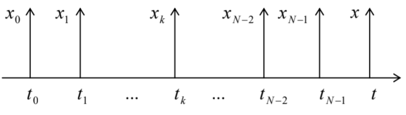 Fig. 5.4. Time partition and coordinate notation at the initial stage of the Feynman path integral’s derivation.
The key Feynman’s breakthrough was the realization that if all intervals are taken similar and sufficiently small, \(t_{k}-t_{k-1}=d \tau \rightarrow 0\), all the partial brackets participating in Eq. (43) may be expressed via the free-particle’s propagator, given by Eq. (2.49), even if the particle is not free, but moves in a stationary potential profile \(U(x)\). To show that, let us use either Eq. (4.175) or Eq. (4.181), which, for a small time interval \(d \tau\), give the same result: \[\hat{u}(\tau+d \tau, \tau)=\exp \left\{-\frac{i}{\hbar} \hat{H} d \tau\right\}=\exp \left\{-\frac{i}{\hbar}\left(\frac{\hat{p}^{2}}{2 m} d \tau+U(\hat{x}) d \tau\right)\right\} .\] Generally, an exponent of a sum of two operators may be treated as that of \(c\)-number arguments, and in particular factored into a product of two exponents, only if the operators commute. (In this case, we can use all the standard algebra for the exponents of \(c\)-number arguments.) In our case, this is not so, because the operator \(\hat{p}^{2} / 2 m\) does not commute with \(\hat{x}\), and hence with \(U(\hat{x})\). However, it may be shown \({ }^{18}\) that for an infinitesimal time interval \(d \tau\), the non-zero commutator \[\left[\frac{\hat{p}^{2}}{2 m} d \tau, U(\hat{x}) d \tau\right] \neq 0,\] proportional to \((d \tau)^{2}\), may be ignored in the first, linear approximation in \(d \tau\). As a result, we may factorize the right-hand side in Eq. (44) by writing \[\hat{u}(\tau+d \tau, \tau)_{d \tau \rightarrow 0} \rightarrow \exp \left\{-\frac{i}{\hbar} \frac{\hat{p}^{2}}{2 m} d \tau\right\} \exp \left\{-\frac{i}{\hbar} U(\hat{x}) d \tau\right\} .\] (This approximation is very much similar in spirit to the trapezoidal-rule approximation in the usual 1D integration, \({ }^{19}\) which in also asymptotically impeachable.)Since the second exponential function on the right-hand side of Eq. (46) commutes with the coordinate operator, we may move it out of each partial bracket participating in Eq. (43), with \(U(x)\) turning into a \(c\)-number function: \[\left\langle x_{\tau+d \tau}|\hat{u}(\tau+d \tau, \tau)| x_{\tau}\right\rangle=\left\langle x_{\tau+d \tau}\left|\exp \left\{-\frac{i}{\hbar} \frac{\hat{p}^{2}}{2 m} d \tau\right\}\right| x_{\tau}\right\rangle \exp \left\{-\frac{i}{\hbar} U(x) d \tau\right\} .\] But the remaining bracket is just the propagator of a free particle, so that for it we may use Eq. (2.49): \[\left\langle x_{\tau+d \tau}\left|\exp \left\{-\frac{i}{\hbar} \frac{\hat{p}^{2}}{2 m} d \tau\right\}\right| x_{\tau}\right\rangle=\left(\frac{m}{2 \pi i \hbar d \tau}\right)^{1 / 2} \exp \left\{i \frac{m(d x)^{2}}{2 \hbar d \tau}\right\} .\] As the result, the full propagator (43) takes the form \[G\left(x, t ; x_{0} t_{0}\right)=\lim _{d \tau \rightarrow 0} \int d x_{N-1} \int d x_{N-2} . . . d x_{1}\left(\frac{m}{2 \pi i \hbar d \tau}\right)^{N / 2} \exp \left\{\sum_{k=1}^{N}\left[i \frac{m(d x)^{2}}{2 \hbar d \tau}-i \frac{U(x)}{\hbar} d \tau\right]\right\} .\] At \(N \rightarrow \infty\) and hence \(d \tau \equiv\left(t-t_{0}\right) / N \rightarrow 0\), the sum under the exponent in this expression may be approximated with the corresponding integral: \[\sum_{k=1}^{N} \frac{i}{\hbar}\left[\frac{m}{2}\left(\frac{d x}{d \tau}\right)^{2}-U(x)\right]_{\tau=t_{k}} d \tau \rightarrow \frac{i}{\hbar} \int_{t_{0}}^{t}\left[\frac{m}{2}\left(\frac{d x}{d \tau}\right)^{2}-U(x)\right] d \tau,\] and the expression in the square brackets is just the particle’s Lagrangian function \(\mathscr{L}^{20}\) The integral of this function over time is the classical action \(S\) calculated along a particular "path" \(x(\tau){ }^{21}\) As a result, defining the (1D) path integral as \[\int(\ldots) D[x(\tau)] \equiv \lim _{d \tau \rightarrow 0 \atop N \rightarrow \infty}\left(\frac{m}{2 \pi i \hbar d \tau}\right)^{N / 2} \int d x_{N-1} \int d x_{N-2} . . \int d x_{1}(\ldots)\] we can bring our result to the following (superficially simple) form: \[G\left(x, t ; x_{0}, t_{0}\right)=\int \exp \left\{\frac{i}{\hbar} s[x(\tau)]\right\} D[x(\tau)] .\] The name "path integral" for the mathematical construct (51a) may be readily explained if we keep the number \(N\) of time intervals large but finite, and also approximate each of the enclosed integrals with a sum over \(M \gg 1\) discrete points along the coordinate axis - see Fig. 5 a.
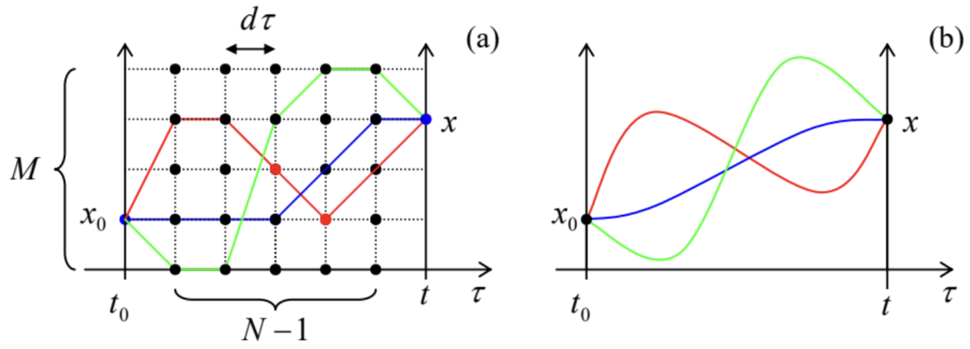 Fig. 5.5. Several 1D classical paths: (a) in the discrete approximation and (b) in the continuous limit.
Then the path integral (51a) is the product of \((N-1)\) sums corresponding to different values of time \(\tau\), each of them with \(M\) terms, each of those representing the function under the integral at a particular spatial point. Multiplying those \((N-1)\) sums, we get a sum of \((N-1) M\) terms, each evaluating the function at a specific spatial-temporal point \([x, \tau]\). These terms may be now grouped to represent all possible different continuous classical paths \(x[\tau]\) from the initial point \(\left[x_{0}, t_{0}\right]\) to the finite point \([x, t]\). It is evident that the last interpretation remains true even in the continuous limit \(N, M \rightarrow \infty-\) see Fig. 5b.
Why does such path representation of the sum make sense? This is because in the classical limit the particle follows just a certain path, corresponding to the minimum of the action \(S\). As a result, for all close trajectories, the difference \(\left(S-S_{\mathrm{cl}}\right)\) is proportional to the square of the deviation from the classical trajectory. Hence, for a quasiclassical motion, with \(\delta_{\mathrm{cl}} \gg \lambda\), there is a bunch of close trajectories, with \(\left(S-S_{\mathrm{cl}}\right)<<\hbar\), that give substantial contributions to the path integral. On the other hand, strongly non-classical trajectories, with \(\left(S-S_{\mathrm{cl}}\right) \gg \hbar\), give phases \(S\) औ rapidly oscillating from one trajectory to the next one, and their contributions to the path integral are averaged out. \({ }^{22}\) As a result, for a quasi-classical motion, the propagator’s exponent may be evaluated on the classical path only: \[G_{\mathrm{cl}} \propto \exp \left\{\frac{i}{\hbar} S_{\mathrm{cl}}\right\}=\exp \left\{\frac{i}{\hbar} \int_{t_{0}}^{t}\left[\frac{m}{2}\left(\frac{d x}{d \tau}\right)^{2}-U(x)\right] d \tau\right\} .\] The sum of the kinetic and potential energies is the full energy \(E\) of the particle, that remains constant for motion in a stationary potential \(U(x)\), so that we may rewrite the expression under this integral as \({ }^{23}\) \[\left[\frac{m}{2}\left(\frac{d x}{d \tau}\right)^{2}-U(x)\right] d \tau=\left[m\left(\frac{d x}{d \tau}\right)^{2}-E\right] d \tau=m \frac{d x}{d \tau} d x-E d \tau\] With this replacement, Eq. (52) yields \[G_{\mathrm{cl}} \propto \exp \left\{\frac{i}{\hbar} \int_{x_{0}}^{x} m \frac{d x}{d \tau} d x\right\} \exp \left\{-\frac{i}{\hbar} E\left(t-t_{0}\right)\right\}=\exp \left\{\frac{i}{\hbar} \int_{x_{0}}^{x} p(x) d x\right\} \exp \left\{-\frac{i}{\hbar} E\left(t-t_{0}\right)\right\},\] where \(p\) is the classical momentum of the particle. But (at least, leaving the pre-exponential factor alone) this is the WKB approximation result that was derived and studied in detail in Chapter 2!
One may question the value of such a complicated calculation, which yields the results that could be readily obtained from Schrödinger’s wave mechanics. Feynman’s approach is indeed not used too often, but it has its merits. First, it has an important philosophical (and hence heuristic) value. Indeed, Eq. (51) may be interpreted by saying that the essence of quantum mechanics is the exploration, by the system, of all possible paths \(x(\tau)\), each of them classical-like, in the sense that the particle’s coordinate \(x\) and velocity \(d x / d \tau\) are exactly defined simultaneously at each point. The resulting contributions to the path integral are added up coherently to form the actual propagator \(G\), and via it, the final probability \(W\) \(\propto|G|^{2}\) of the particle’s propagation from \(\left[x_{0}, t_{0}\right]\) to \([x, t]\). As the scale of the action \(S\) of the motion decreases and becomes comparable to \(\hbar\), more and more paths produce substantial contributions to this sum, and hence to \(W\), providing a larger and larger difference between the quantum and classical properties of the system.
Second, the path integral provides a justification for some simple explanations of quantum phenomena. A typical example is the quantum interference effects discussed in Sec. \(3.1-\) see, e.g., Fig. \(3.1\) and the corresponding text. At that discussion, we used the Huygens principle to argue that at the two-slit interference, the WKB approximation might be restricted to contributions from two paths that pass through different slits, but otherwise consisting of straight-line segments. To have another look at that assumption, let us generalize the path integral to multi-dimensional geometries. Fortunately, the simple structure of Eq. (51b) makes such generalization virtually evident: \[G\left(\mathbf{r}, t ; \mathbf{r}_{0}, t_{0}\right)=\int \exp \left\{\frac{i}{\hbar} S[\mathbf{r}(\tau)]\right\} D[\mathbf{r}(\tau)], \quad S \equiv \int_{t_{0}}^{t} \mathscr{L}\left(\mathbf{r}, \frac{d \mathbf{r}}{d \tau}\right) d \tau=\int_{t_{0}}^{t}\left[\frac{m}{2}\left(\frac{d \mathbf{r}}{d \tau}\right)^{2}-U(\mathbf{r})\right] d \tau .\] where the definition (51a) of the path integral should be also modified correspondingly. (I will not go into these technical details.) For the Young-type experiment (Fig. 3.1), where a classical particle could reach the detector only after passing through one of the slits, the classical paths are the straight-line segments shown in Fig. 3.1, and if they are much longer than the de Broglie wavelength, the propagator may be well approximated by the sum of two integrals of \(\mathscr{L} d \tau=i \mathbf{p}(\mathbf{r}) \cdot d \mathbf{r} / \hbar-\) as it was done in \(\operatorname{Sec} .3 .1\).
Last but not least, the path integral allows simple solutions to some problems that would be hard to obtain by other methods. As the simplest example, let us consider the problem of tunneling in multidimensional space, sketched in Fig. 6 for the \(2 \mathrm{D}\) case \(-\) just for the graphics’ simplicity. Here, the potential profile \(U(x, y)\) has a saddle-like shape. (Another helpful image is a mountain path between two summits, in Fig. 6 located on the top and at the bottom of the shown region.) A particle of energy \(E\) may move classically in the left and right regions with \(U(x, y)<E\), but if \(E\) is not sufficiently high, it can pass from one of these regions to another one only via the quantum-mechanical tunneling under the pass. Let us calculate the transparency of this potential barrier in the WKB approximation, ignoring the possible pre-exponential factor. \({ }^{24}\)
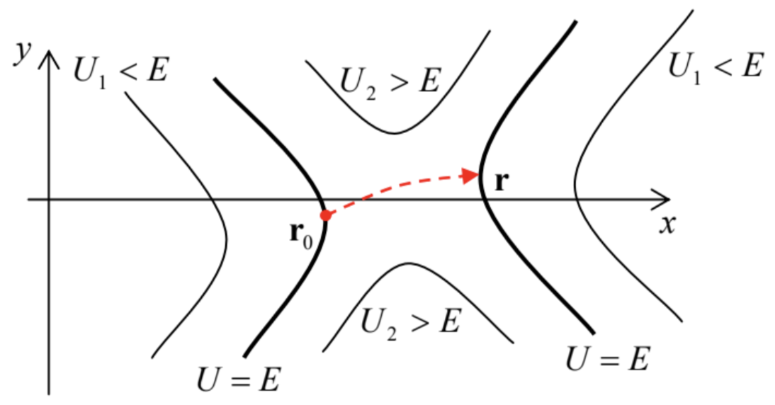
According to the evident multi-dimensional generalization Eq. (54), for the classically forbidden region, where \(E<U(x, y)\), and hence \(\mathbf{p}(\mathbf{r}) / \hbar=i \boldsymbol{\kappa}(\mathbf{r})\), the contributions to the propagator (55) are proportional to \[e^{-I} \exp \left\{-\frac{i}{\hbar} E\left(t-t_{0}\right)\right\}, \quad \text { where } I \equiv \int_{\mathbf{r}_{0}}^{\mathbf{r}} \boldsymbol{\kappa}(\mathbf{r}) \cdot d \mathbf{r}\] where \(\kappa \equiv \kappa\) may be calculated just in the \(1 \mathrm{D}\) case \(-\) cf. Eq. \((2.97)\) : \[\frac{\hbar^{2} \kappa^{2}(\mathbf{r})}{2 m}=U(\mathbf{r})-E \text {. }\] Hence the path integral in this region is much simpler than in the classically allowed region, because the spatial exponents are purely real and there is no complex interference between them. Due to the minus sign before \(I\) in the exponent (56), the largest contribution to \(G\) evidently comes from the trajectory (or a narrow bundle of close trajectories) for which the integral \(I\) has the smallest value, so that the barrier transparency may be calculated as \[\mathscr{T} \approx|G|^{2} \approx e^{-2 I} \equiv \exp \left\{-2 \int_{\mathbf{r}_{0}}^{\mathbf{r}} \boldsymbol{\kappa}\left(\mathbf{r}^{\prime}\right) \cdot d \mathbf{r}^{\prime}\right\},\] where \(\mathbf{r}\) and \(\mathbf{r}_{0}\) are certain points on the opposite classical turning-point surfaces: \(U(\mathbf{r})=U\left(\mathbf{r}_{0}\right)=E-\) see Fig. 6 .
Thus the barrier transparency problem is reduced to finding the trajectory (including the points \(\mathbf{r}\) and \(\mathbf{r}_{0}\) ) that connects the two surfaces and minimizes the functional \(I\). This is of course a well-known problem of the calculus of variations, \({ }^{25}\) but it is interesting that the path integral provides a simple alternative way of solving it. Let us consider an auxiliary problem of particle’s motion in the potential profile \(U_{\text {inv }}(\mathbf{r})\) that is inverted relative to the particle’s energy \(E\), i.e. is defined by the following equality: \[U_{\text {inv }}(\mathbf{r})-E \equiv E-U(\mathbf{r})\] As was discussed above, at fixed energy \(E\), the path integral for the WKB motion in the classically allowed region of potential \(U_{\text {inv }}(x, y)\) (that coincides with the classically forbidden region of the original problem) is dominated by the classical trajectory corresponding to the minimum of \[S_{\text {inv }}=\int_{\mathbf{r}_{0}}^{\mathbf{r}} \mathbf{p}_{\text {inv }}\left(\mathbf{r}^{\prime}\right) \cdot d \mathbf{r}^{\prime}=\hbar \int_{\mathbf{r}_{0}}^{\mathbf{r}} \mathbf{k}_{\text {inv }}\left(\mathbf{r}^{\prime}\right) \cdot d \mathbf{r},\] where \(\mathbf{k}_{\text {inv }}\) should be determined from the WKB relation \[\frac{\hbar^{2} k_{\text {inv }}^{2}(\mathbf{r})}{2 m} \equiv E-U_{\text {inv }}(\mathbf{r}) .\] But comparing Eqs. (57), (59), and (61), we see that \(\mathbf{k}_{\text {inv }}=\mathbf{\kappa}\) at each point! This means that the tunneling path (in the WKB limit) corresponds to the classical (so-called instanton \({ }^{26}\) ) trajectory of the same particle moving in the inverted potential \(U_{\text {inv }}(\mathbf{r})\). If the initial point \(\mathbf{r}_{0}\) is fixed, this trajectory may be readily found by the means of classical mechanics. (Note that the initial kinetic energy, and hence the initial velocity of the instanton launched from point \(\mathbf{r}_{0}\) should be zero because by the classical turning point definition, \(U_{\text {inv }}\left(\mathbf{r}_{0}\right)=U\left(\mathbf{r}_{0}\right)=E\).) Thus the problem is further reduced to a simpler task of maximizing the transparency (58) by choosing the optimal position of \(\mathbf{r}_{0}\) on the equipotential surface \(U\left(\mathbf{r}_{0}\right)=E-\) see Fig. 6 . Moreover, for many symmetric potentials, the position of this point may be readily guessed even without calculations - as it is in Problems 6 and 7, left for the reader’s exercise.
Note that besides the calculation of the potential barrier’s transparency, the instanton trajectory has one more important implication: the so-called traversal time \(\tau_{\mathrm{t}}\) of the classical motion along it, from the point \(\mathbf{r}_{0}\) to the point \(\mathbf{r}\), in the inverted potential defined by Eq. (59), plays the role of the most important (though not the only one) time scale of the particle’s tunneling under the barrier. \({ }^{27}\)
\({ }^{16}\) This formulation was developed in 1948 by Richard Phillips Feynman. (According to his memories, this work was motivated by a "mysterious" remark by P. Dirac in his pioneering 1930 textbook on quantum mechanics.)
\({ }^{17}\) A more thorough discussion of the path-integral approach may be found in the famous text by R. Feynman and A. Hibbs, Quantum Mechanics and Path Integrals, first published in 1965. (For its latest edition by Dover in 2010, the book was emended by D. Styler.) For a more recent monograph, which reviews more applications, see L. Schulman, Techniques and Applications of Path Integration, Wiley, \(1981 .\)
\({ }^{18}\) This is exactly the corner I am going to cut because a strict mathematical proof of this (intuitively evident) statement would take more time/space than I can afford.
\({ }^{19}\) See, e.g., MA Eq. (5.2).
\({ }^{20}\) See, e.g., CM Sec. 2.1
\({ }^{21}\) See, e.g., CM Sec. 10.3.
\({ }^{22}\) This fact may be proved by expanding the difference \(\left(S-S_{\mathrm{cl}}\right)\) in the Taylor series in the path variation (leaving only the leading quadratic terms) and working out the resulting Gaussian integrals. This integration, together with the pre-exponential coefficient in Eq. (51a), gives exactly the pre-exponential factor that we have already found refining the WKB approximation in Sec. 2.4.
\({ }^{23}\) The same trick is often used in analytical classical mechanics - say, for proving the Hamilton principle, and for the derivation of the Hamilton - Jacobi equations (see, e.g., CM Secs. 10.3-4).
\({ }^{24}\) Actually, one can argue that the pre-exponential factor should be close to 1, just like in Eq. (2.117), especially if the potential is smooth, in the sense of Eq. (2.107), in all spatial directions. (Let me remind the reader that for most practical applications of quantum tunneling, the pre-exponential factor is of minor importance.)
\({ }^{25}\) For a concise introduction to the field see, e.g., I. Gelfand and S. Fomin, Calculus of Variations, Dover, 2000, or L. Elsgolc, Calculus of Variations, Dover, \(2007 .\)
\({ }^{26}\) In the quantum field theory, the instanton concept may be formulated somewhat differently, and has more complex applications - see, e.g. R. Rajaraman, Solitons and Instantons, North-Holland, \(1987 .\)
\({ }^{27}\) For more on this interesting issue see, e.g., M. Buttiker and R. Landauer, Phys. Rev. Lett. 49, 1739 (1982), and references therein.