9.1: Electromagnetic Field Quantization

Classical physics gives us \(^{3}\) the following general relativistic relation between the momentum \(\mathbf{p}\) and energy \(E\) of a free particle with rest mass \(m\), which may be simplified in two limits - non-relativistic and ultra-relativistic: \[E=\left[(p c)^{2}+\left(m c^{2}\right)^{2}\right]^{1 / 2} \rightarrow \begin{cases}m c^{2}+p^{2} / 2 m, & \text { for } p<<m c \\ p c, & \text { for } p>>m c\end{cases}\] In both limits, the transfer from classical to quantum mechanics is easier than in the arbitrary case. Since all the previous part of this course was committed to the first, non-relativistic limit, I will now jump to a brief discussion of the ultra-relativistic limit \(p>>m c\), for a particular but very important system - the electromagnetic field. Since the excitations of this field, called photons, are currently believed to have zero rest mass \(m,{ }^{4}\) the ultra-relativistic relation \(E=p c\) is exactly valid for any photon energy \(E\), and the quantization scheme is rather straightforward.

As usual, the quantization has to be based on the classical theory of the system - in this case, the Maxwell equations. As the simplest case, let us consider the electromagnetic field inside a finite freespace volume limited by ideal walls, which reflect incident waves perfectly. \({ }^{5}\) Inside the volume, the Maxwell equations give a simple wave equation \({ }^{6}\) for the electric field \[\nabla^{2} \mathscr{E}-\frac{1}{c^{2}} \frac{\partial^{2} \mathscr{E}}{\partial t^{2}}=0,\] and an absolutely similar equation for the magnetic field \(\mathscr{B}\). We may look for the general solution of Eq. (2) in the variable-separating form \[\mathscr{E}(\mathbf{r}, t)=\sum_{j} p_{j}(t) \mathbf{e}_{j}(\mathbf{r}) .\] Physically, each term of this sum is a standing wave whose spatial distribution and polarization ("mode") are described by the vector function \(\mathbf{e}_{j}(\mathbf{r})\), while the temporal dynamics, by the function \(p_{j}(t)\). Plugging an arbitrary term of this sum into Eq. (2), and separating the variables exactly as we did, for example, in the Schrödinger equation in Sec. 1.5, we get \[\frac{\nabla^{2} \mathbf{e}_{j}}{\mathbf{e}_{j}}=\frac{1}{c^{2}} \frac{\ddot{p}_{j}}{p_{j}}=\text { const } \equiv-k_{j}^{2},\] so that the spatial distribution of the mode satisfies the 3D Helmholtz equation: \[\nabla^{2} \mathbf{e}_{j}+k_{j}^{2} \mathbf{e}_{j}=0\] The set of solutions of this equation, with appropriate boundary conditions, determines the set of the functions \(\mathbf{e}_{j}\), and simultaneously the spectrum of the wave number magnitudes \(k_{j}\). The latter values determine the mode eigenfrequencies, following from Eq. (4): \[\ddot{p}_{j}+\omega_{j}^{2} p_{j}=0, \quad \text { with } \omega_{j} \equiv k_{j} c .\] There is a big philosophical difference between the quantum-mechanical approach to Eqs. (5) and (6), despite their single origin (4). The first (Helmholtz) equation may be rather difficult to solve in realistic geometries, \({ }^{7}\) but it remains intact in the basic quantum electrodynamics, with the scalar components of the vector functions \(\mathbf{e}_{j}(\mathbf{r})\) still treated (at each point \(\mathbf{r}\) ) as \(c\)-numbers. In contrast, the classical Eq. (6) is readily solvable (giving sinusoidal oscillations with frequency \(\omega_{j}\) ), but this is exactly where we can make the transfer to quantum mechanics, because we already know how to quantize a mechanical 1D harmonic oscillator, which in classics obeys the same equation.

As usual, we need to start with the appropriate Hamiltonian - the operator corresponding to the classical Hamiltonian function \(H\) of the proper set of generalized coordinates and momenta. The electromagnetic field’s Hamiltonian function (which in this case coincides with the field’s energy) is \(^{8}\) \[H=\int d^{3} r\left(\frac{\varepsilon_{0} \mathscr{E}^{2}}{2}+\frac{\mathscr{B}^{2}}{2 \mu_{0}}\right) .\] Let us represent the magnetic field in a form similar to Eq. (3), \({ }^{9}\) \[\mathscr{B}(\mathbf{r}, t)=-\sum_{j} \omega_{j} q_{j}(t) \mathbf{b}_{j}(\mathbf{r}) .\] Since, according to the Maxwell equations, in our case the magnetic field satisfies the equation similar to Eq. (2), the time-dependent amplitude \(q_{j}\) of each of its modes \(\mathbf{b}_{j}(\mathbf{r})\) obeys an equation similar to Eq. (6), i.e. in the classical theory also changes in time sinusoidally, with the same frequency \(\omega_{j}\). Plugging Eqs. (3) and (8) into Eq. (7), we may recast it as \[H=\sum_{j}\left[\frac{p_{j}^{2}}{2} \int \varepsilon_{0} e_{j}^{2}(\mathbf{r}) d^{3} r+\frac{\omega_{j}^{2} q_{j}^{2}}{2} \int \frac{1}{\mu_{0}} b_{j}^{2}(\mathbf{r}) d^{3} r\right] .\] Since the distribution of constant factors between two multiplication operands in each term of Eq. (3) is so far arbitrary, we may fix it by requiring the first integral in Eq. (9) to equal 1. It is straightforward to check that according to the Maxwell equations, which give a specific relation between vectors \(\mathscr{E}\) and \(\mathscr{B},{ }^{10}\) this normalization makes the second integral in Eq. (9) equal 1 as well, and Eq. (9) becomes \[H=\sum_{j} H_{j}, \quad H_{j}=\frac{p_{j}^{2}}{2}+\frac{\omega_{j}^{2} q_{j}^{2}}{2} .\] Note that that \(p_{j}\) is the legitimate generalized momentum corresponding to the generalized coordinate \(q_{\mathrm{j}}\), because it is equal to \(\partial L / \partial \dot{q}_{j}\), where \(L\) is the Lagrangian function of the field - see EM Eq. (9.217): \[L=\int d^{3} r\left(\frac{\varepsilon_{0} \mathscr{E}^{2}}{2}-\frac{\mathscr{R}^{2}}{2 \mu_{0}}\right)=\sum_{j} L_{j}, \quad L_{j}=\frac{p_{j}^{2}}{2}-\frac{\omega_{j}^{2} q_{j}^{2}}{2} .\] Hence we can carry out the standard quantization procedure, namely declare \(H_{j}, p_{j}\), and \(q_{j}\) the quantum-mechanical operators related exactly as in Eq. (10a), \[\hat{H}_{j}=\frac{\hat{p}_{j}^{2}}{2}+\frac{\omega_{j}^{2} \hat{q}_{j}^{2}}{2} .\] We see that this Hamiltonian coincides with that of a 1D harmonic oscillator with the mass \(m_{j}\) formally equal to \(1,{ }^{11}\) and the eigenfrequency equal to \(\omega_{j}\). However, in order to use Eq. (11) in the general Eq. (4.199) for the time evolution of Heisenberg-picture operators \(\hat{p}_{j}\) and \(\hat{q}_{j}\), we need to know the commutation relation between these operators. To find them, let us calculate the Poisson bracket (4.204) for the functions \(A=q_{j}\), and \(B=p_{j^{\prime \prime}}\), taking into account that in the classical Hamiltonian mechanics, all generalized coordinates \(q_{j}\) and the corresponding momenta \(p_{j}\) have to be considered independent arguments of \(H\), only one term (with \(j=j^{\prime}=j^{\prime \prime}\) ) in only one of the sums (12) (namely, with \(j^{\prime}=j^{\prime \prime}\) ), gives a non-zero value \((-1)\), so that

\[\ \left\{q_{j^{\prime},} p_{j^{\prime\prime}}\right\}_{\mathrm{P}} \equiv \sum_{j}\left(\frac{\partial q_{j^{\prime}}}{\partial p_{j}} \frac{\partial p_{j^{\prime \prime}}}{\partial q_{j}}-\frac{\partial q_{j^{\prime}}}{\partial q_{j}} \frac{\partial p_{j^{\prime \prime}}}{\partial p_{j^{}}}\right)=-\delta_{j^{\prime} j^{\prime \prime}}.\]

Hence, according to the general quantization rule (4.205), the commutation relation of the operators corresponding to \(q_{j}\), and \(p_{j}\), is \[\left[\hat{q}_{j^{\prime}}, \hat{p}_{j^{\prime \prime}}\right]=i \hbar \delta_{j j^{\prime \prime}},\] i.e. is exactly the same as for the usual Cartesian components of the radius-vector and momentum of a mechanical particle \(-\) see Eq. (2.14).

As the reader already knows, Eqs. (11) and (13) open for us several alternative ways to proceed:

(i) Use the Schrödinger-picture wave mechanics based on wavefunctions \(\Psi_{j}\left(q_{j}, t\right)\). As we know from Sec. 2.9, this way is inconvenient for most tasks, because the eigenfunctions of the harmonic oscillator are rather clumsy.

(ii) A substantially better way (for the harmonic oscillator case) is to write the equations of the time evolution of the operators \(\hat{q}_{j}(t)\) and \(\hat{p}_{j}(t)\) in the Heisenberg picture of quantum dynamics.

(iii) An even more convenient approach is to use equations similar to Eqs. (5.65) to decompose the Heisenberg operators \(\hat{q}_{j}(t)\) and \(\hat{p}_{j}(t)\) into the creation-annihilation operators \(\hat{a}_{j}^{\dagger}(t)\) and \(\hat{a}_{j}(t)\), and work with these operators.

In this chapter, I will mostly use the last route. Replacing \(m\) with \(m_{j} \equiv 1\), and \(\omega_{0}\) with \(\omega_{j}\), the last forms of Eqs. (5.65) become \[\hat{a}_{j}=\left(\frac{\omega_{j}}{2 \hbar}\right)^{1 / 2}\left(\hat{q}_{j}+i \frac{\hat{p}_{j}}{\omega_{j}}\right), \quad \hat{a}_{j}^{\dagger}=\left(\frac{\omega_{j}}{2 \hbar}\right)^{1 / 2}\left(\hat{q}_{j}-i \frac{\hat{p}_{j}}{\omega_{j}}\right) .\] Due to Eq. (13), the creation-annihilation operators obey the commutation similar to Eq. (5.68), \[\left[\hat{a}_{j}, \hat{a}_{j^{\prime}}^{\dagger}\right]=\hat{I} \delta_{i j^{\prime}} .\] As a result, according to Eqs. (3) and (8), the quantum-mechanical operators of the electric and magnetic fields are sums over all field oscillators: \[\begin{aligned} &\hat{\mathscr{E}}(\mathbf{r}, t)=i \sum_{j}\left(\frac{\hbar \omega_{j}}{2}\right)^{1 / 2} \mathbf{e}_{j}(\mathbf{r})\left(\hat{a}_{j}^{\dagger}-\hat{a}_{j}\right), \\ &\hat{\mathscr{B}}(\mathbf{r}, t)=\sum_{j}\left(\frac{\hbar \omega_{j}}{2}\right)^{1 / 2} \mathbf{b}_{j}(\mathbf{r})\left(\hat{a}_{j}^{\dagger}+\hat{a}_{j}\right), \end{aligned}\] and Eq. (11) for the \(j^{\text {th }}\) mode’s Hamiltonian becomes \[\hat{H}_{j}=\hbar \omega_{j}\left(\hat{a}_{j}^{\dagger} \hat{a}_{j}+\frac{1}{2} \hat{I}\right)=\hbar \omega_{j}\left(\hat{n}_{j}+\frac{1}{2} \hat{I}\right), \quad \text { with } \hat{n}_{j} \equiv \hat{a}_{j}^{\dagger} \hat{a}_{j},\] absolutely similar to Eq. (5.72) for a mechanical oscillator.

Now comes a very important conceptual step. From Sec. \(5.4\) we know that the eigenfunctions (Fock states) \(n_{j}\) of the Hamiltonian (17) have energies \[E_{j}=\hbar \omega_{j}\left(n_{j}+\frac{1}{2}\right), \quad n_{j}=0,1,2, \ldots\] and, according to Eq. (5.89), the operators \(\hat{a}_{j}^{\dagger}\) and \(\hat{a}_{j}\) act on the eigenkets of these partial states as \[\hat{a}_{j}\left|n_{j}\right\rangle=\left(n_{j}\right)^{1 / 2}\left|n_{j}-1\right\rangle, \quad \hat{a}_{j}^{\dagger}\left|n_{j}\right\rangle=\left(n_{j}+1\right)^{1 / 2}\left|n_{j}+1\right\rangle,\] regardless of the quantum states of other modes. These rules coincide with the definitions (8.64) and (8.68) of bosonic creation-annihilation operators, and hence their action may be considered as the creation/annihilation of certain bosons. Such a "particle" (actually, an excitation, with energy \(\hbar \omega_{j}\), of an electromagnetic field oscillator) is exactly what is, strictly speaking, called a photon. Note immediately that according to Eq. (16), such an excitation does not change the spatial distribution of the \(j^{\text {th }}\) mode of the field. So, such a "global" photon is an excitation created simultaneously at all points of the field confinement region.

If this picture is too contrary to the intuitive image of a particle, please recall that in Chapter 2 , we discussed a similar situation with the fundamental solutions of the Schrödinger equation of a free non-relativistic particle: they represent sinusoidal de Broglie waves existing simultaneously in all points of the particle confinement region. The (partial :-) reconciliation with the classical picture of a moving particle might be obtained by using the linear superposition principle to assemble a quasi-localized wave packet, as a group of sinusoidal waves with close wave numbers. Very similarly, we may form a similar wave packet using a linear superposition of the "global" photons with close values of \(\mathbf{k}_{j}\) (and hence \(\omega_{j}\) ), to form a quasi-localized photon. An additional simplification here is that the dispersion relation for electromagnetic waves (at least in free space) is linear: \[\frac{\partial \omega_{j}}{\partial k_{j}}=c=\mathrm{const}, \quad \text { i.e. } \frac{\partial^{2} \omega_{j}}{\partial k_{j}{ }^{2}}=0\] so that, according to Eq. (2.39a), the electromagnetic wave packets (i.e. space-localized photons) do not spread out during their propagation. Note also that due to the fundamental classical relations \(\mathbf{p}=\mathbf{n} E / c\) for the linear momentum of the traveling electromagnetic wave packet of energy \(E\), propagating along the direction \(\mathbf{n} \equiv \mathbf{k} / k\), and \(\mathbf{L}=\pm \mathbf{n} E / \omega_{j}\) for its angular momentum, \({ }^{12}\) such photon may be prescribed the linear momentum \(\mathbf{p}=\mathbf{n} \hbar \omega_{j} / c \equiv \hbar \mathbf{k}\) and the angular momentum \(\mathbf{L}=\pm \mathbf{n} \hbar\), with the sign depending on the direction of its circular polarization ("helicity").

This electromagnetic field quantization scheme should look very straightforward, but it raises an important conceptual issue of the ground state energy. Indeed, Eq. (18) implies that the total groundstate (i.e., the lowest) energy of the field is \[E_{\mathrm{g}}=\sum_{j}\left(E_{\mathrm{g}}\right)_{j}=\sum_{j} \frac{\hbar \omega_{j}}{2} .\] Since for any realistic model of the field-confining volume, either infinite or not, the density of electromagnetic field modes only grows with frequency, \({ }^{13}\) this sum diverges on its upper limit, leading to infinite ground-state energy per unit volume. This infinite-energy paradox cannot be dismissed by declaring the ground-state energy of field oscillators unobservable, because this would contradict numerous experimental observations \(-\) starting perhaps from the famous Casimir effect. \({ }^{14}\) The conceptually simplest implementation of this effect involves two parallel, perfectly conducting plates of area \(A\), separated by a vacuum gap of thickness \(t<<A^{1 / 2}\) (Fig. 1).

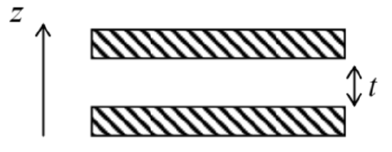Fig. 9.1. The simplest geometry of the Casimir effect manifestation.

Rather counter-intuitively, the plates attract each other with a force \(F\) proportional to the area \(A\) and rapidly increasing with the decrease of \(t\), even in the absence of any explicit electromagnetic field sources. The effect’s explanation is that the energy of each electromagnetic field mode, including its ground-state energy, exerts average pressure, \[\left\langle\mathcal{P}_{j}\right\rangle=-\frac{\partial E_{j}}{\partial V},\] on the walls constraining it to volume \(V\). While the field’s pressure on the external surfaces on the plates is due to the contributions (22) of all free-space modes, with arbitrary values of \(k_{z}\) (the \(z\)-component of the wave vector \(\mathbf{k}_{j}\) ), in the gap between the plates the spectrum of \(k_{z}\) is limited to the multiples of \(\pi / t\), so that the pressure on the internal surfaces is lower. This is why the net force exerted on the plates may be calculated as the sum of the contributions (22) from all "missing" low-frequency modes in the gap, with the minus sign. In the simplest model when the plates are made of an ideal conductor, which provides boundary conditions \(\mathscr{E}_{\tau}=\mathscr{B}_{n}=0\) on their surfaces, \({ }^{15}\) such calculation is quite straightforward (and is hence left for the reader’s exercise), and its result is \[F=-\frac{\pi^{2} A \hbar c}{240 t^{4}} .\] Note that for such calculation, the high-frequency divergence of Eq. (21) is not important, because it participates in the forces exerted on all surfaces of each plate, and cancels out from the net pressure. In this way, the Casimir effect not only confirms Eq. (21), but also teaches us an important lesson on how to deal with the divergences of such sums at \(\omega_{j} \rightarrow \infty\). The lesson is: just get accustomed to the idea that the divergence exists, and ignore this fact while you can, i.e. if the final result you are interested in is finite. However, for some more complex problems of quantum electrodynamics (and the quantum theory of any other fields), this simplest approach becomes impossible, and then more complex, renormalization techniques become necessary. For their study, I have to refer the reader to a quantum field theory course \(-\) see the references at the end of this chapter.

---

\({ }^{1}\) Note that some material covered in this chapter is frequently taught as a part of the quantum field theory. I will focus on the most important results that may be obtained without starting the heavy engines of that theory.

\({ }^{2}\) The described approach was pioneered by the same P. A. M. Dirac as early as \(1927 .\)

\({ }^{3}\) See, e.g., EM Chapter \(9 .\)

\({ }^{4}\) By now this fact has been verified experimentally with an accuracy of at least \(\sim 10^{-22} m_{\mathrm{e}}-\) see \(\mathrm{S}\). Eidelman et al., Phys. Lett. B 592, 1 (2004).

\({ }^{5}\) In the case of finite energy absorption in the walls, or in the wave propagation media (say, described by complex constants \(\varepsilon\) and \(\mu\) ), the system is not energy-conserving (Hamiltonian), i.e. interacts with some dissipative environment. Specific cases of such interaction will be considered in Sections 2 and 3 below.

\({ }^{6}\) See, e.g., EM Eq. (7.3), for the particular case \(\varepsilon=\varepsilon_{0}, \mu=\mu_{0}\), so that \(v^{2} \equiv 1 / \varepsilon \mu=1 / \varepsilon_{0} \mu_{0} \equiv c^{2}\).

\({ }^{7}\) See, e.g., various problems discussed in EM Chapter 7, especially in Sec. 7.9.

\({ }^{8}\) See, e.g., EM Sec. 9.8, in particular, Eq. (9.225). Here I am using SI units, with \(\varepsilon_{0} \mu_{0} \equiv c^{-2}\); in the Gaussian units, the coefficients \(\varepsilon_{0}\) and \(\mu_{0}\) disappear, but there is an additional common factor \(1 / 4 \pi\) in the equation for energy. However, if we modify the normalization conditions (see below) accordingly, all the subsequent results, starting from Eq. (10), look similar in any system of units.

\({ }^{9}\) Here I am using the letter \(q_{j}\), instead of \(x_{j}\), for the generalized coordinate of the field oscillator, in order to emphasize the difference between the former variable, and one of the Cartesian coordinates, i.e. one of the arguments of the \(c\)-number functions \(\mathbf{e}\) and \(\mathbf{b}\).

\({ }^{10}\) See, e.g., EM Eq. (7.6).

\({ }^{11}\) Selecting a different normalization of the functions \(\mathbf{e}_{j}(\mathbf{r})\) and \(\mathbf{b}_{j}(\mathbf{r})\), we could readily arrange any value of \(m_{j}\), and the choice corresponding to \(m_{j}=1\) is the best one just for the notation simplicity.

\({ }^{12}\) See, e.g., EM Sections \(7.7\) and \(9.8\).

\({ }^{13}\) See, e.g., Eq. (1.1), which is similar to Eq. (1.90) for the de Broglie waves, derived in Sec. 1.7.

\({ }^{14}\) This effect was predicted in 1948 by Hendrik Casimir and Dirk Polder, and confirmed semi-quantitatively in experiments by M. Sparnaay, Nature 180,334 (1957). After this, and several other experiments, a decisive error bar reduction (to about \(\sim 5 \%\) ), providing a quantitative confirmation of the Casimir formula (23), was achieved by S. Lamoreaux, Phys. Rev. Lett. \(\mathbf{7 8}, 5\) (1997) and by U. Mohideen and A. Roy, Phys. Rev. Lett. 81, 004549 (1998). Note also that there are other experimental confirmations of the reality of the ground-state electromagnetic field, including, for example, the experiments by R. Koch et al. already discussed in Sec. \(7.5\), and the recent spectacular direct observations by C. Riek et al., Science 350, 420 (2015).

\({ }^{15}\) For realistic conductors, the reduction of \(t\) below \(\sim 1 \mu \mathrm{m}\) causes significant deviations from this simple model, and hence from Eq. (23). The reason is that for gaps so narrow, the depth of field penetration into the conductors (see, e.g., EM Sec. 6.2), at the important frequencies \(\omega \sim c / t\), becomes comparable with \(t\), and an adequate theory of the Casimir effect has to involve a certain model of the penetration. (It is curious that in-depth analyses of this problem, pioneered in 1956 by E. Lifshitz, have revealed a deep relation between the Casimir effect and the London dispersion force which was the subject of Problems \(3.16,5.15\), and \(6.18\) - for a review see, e.g., either I. Dzhyaloshinskii et al., Sov. Phys. Uspekhi 4, 153 (1961), or K. Milton, The Casimir Effect, World Scientific, 2001. Recent experiments in the \(100 \mathrm{~nm}-2 \mu \mathrm{m}\) range of \(t\), with an accuracy better than \(1 \%\), have allowed not only to observe the effects of field penetration on the Casimir force, but even to make a selection between some approximate models of the penetration - see D. Garcia-Sanchez et al., Phys. Rev. Lett. 109, 027202 (2012).