2.12: Entropy of Mixing and the Gibbs Paradox
( \newcommand{\kernel}{\mathrm{null}\,}\)
\( \newcommand\Dalpha
Callstack:
    at (Template:MathJaxArovas), /content/body/div/p[1]/span[1], line 1, column 1
    at template()
    at (Bookshelves/Thermodynamics_and_Statistical_Mechanics/Book:_Thermodynamics_and_Statistical_Mechanics_(Arovas)/02:_Thermodynamics/2.12:_Entropy_of_Mixing_and_the_Gibbs_Paradox), /content/body/p/span, line 1, column 23
\( \newcommand\Dbeta
Callstack:
    at (Template:MathJaxArovas), /content/body/div/p[1]/span[2], line 1, column 1
    at template()
    at (Bookshelves/Thermodynamics_and_Statistical_Mechanics/Book:_Thermodynamics_and_Statistical_Mechanics_(Arovas)/02:_Thermodynamics/2.12:_Entropy_of_Mixing_and_the_Gibbs_Paradox), /content/body/p/span, line 1, column 23
\( \newcommand\Dgamma
Callstack:
    at (Template:MathJaxArovas), /content/body/div/p[1]/span[3], line 1, column 1
    at template()
    at (Bookshelves/Thermodynamics_and_Statistical_Mechanics/Book:_Thermodynamics_and_Statistical_Mechanics_(Arovas)/02:_Thermodynamics/2.12:_Entropy_of_Mixing_and_the_Gibbs_Paradox), /content/body/p/span, line 1, column 23
\( \newcommand\Ddelta
Callstack:
    at (Template:MathJaxArovas), /content/body/div/p[1]/span[4], line 1, column 1
    at template()
    at (Bookshelves/Thermodynamics_and_Statistical_Mechanics/Book:_Thermodynamics_and_Statistical_Mechanics_(Arovas)/02:_Thermodynamics/2.12:_Entropy_of_Mixing_and_the_Gibbs_Paradox), /content/body/p/span, line 1, column 23
\( \newcommand\Depsilon
Callstack:
    at (Template:MathJaxArovas), /content/body/div/p[1]/span[5], line 1, column 1
    at template()
    at (Bookshelves/Thermodynamics_and_Statistical_Mechanics/Book:_Thermodynamics_and_Statistical_Mechanics_(Arovas)/02:_Thermodynamics/2.12:_Entropy_of_Mixing_and_the_Gibbs_Paradox), /content/body/p/span, line 1, column 23
\( \newcommand\Dvarepsilon
Callstack:
    at (Template:MathJaxArovas), /content/body/div/p[1]/span[6], line 1, column 1
    at template()
    at (Bookshelves/Thermodynamics_and_Statistical_Mechanics/Book:_Thermodynamics_and_Statistical_Mechanics_(Arovas)/02:_Thermodynamics/2.12:_Entropy_of_Mixing_and_the_Gibbs_Paradox), /content/body/p/span, line 1, column 23
\( \newcommand\Dzeta
Callstack:
    at (Template:MathJaxArovas), /content/body/div/p[1]/span[7], line 1, column 1
    at template()
    at (Bookshelves/Thermodynamics_and_Statistical_Mechanics/Book:_Thermodynamics_and_Statistical_Mechanics_(Arovas)/02:_Thermodynamics/2.12:_Entropy_of_Mixing_and_the_Gibbs_Paradox), /content/body/p/span, line 1, column 23
\( \newcommand\Deta
Callstack:
    at (Template:MathJaxArovas), /content/body/div/p[1]/span[8], line 1, column 1
    at template()
    at (Bookshelves/Thermodynamics_and_Statistical_Mechanics/Book:_Thermodynamics_and_Statistical_Mechanics_(Arovas)/02:_Thermodynamics/2.12:_Entropy_of_Mixing_and_the_Gibbs_Paradox), /content/body/p/span, line 1, column 23
\( \newcommand\Dtheta
Callstack:
    at (Template:MathJaxArovas), /content/body/div/p[1]/span[9], line 1, column 1
    at template()
    at (Bookshelves/Thermodynamics_and_Statistical_Mechanics/Book:_Thermodynamics_and_Statistical_Mechanics_(Arovas)/02:_Thermodynamics/2.12:_Entropy_of_Mixing_and_the_Gibbs_Paradox), /content/body/p/span, line 1, column 23
\( \newcommand\Dvartheta
Callstack:
    at (Template:MathJaxArovas), /content/body/div/p[1]/span[10], line 1, column 1
    at template()
    at (Bookshelves/Thermodynamics_and_Statistical_Mechanics/Book:_Thermodynamics_and_Statistical_Mechanics_(Arovas)/02:_Thermodynamics/2.12:_Entropy_of_Mixing_and_the_Gibbs_Paradox), /content/body/p/span, line 1, column 23
\( \newcommand\Diota
Callstack:
    at (Template:MathJaxArovas), /content/body/div/p[1]/span[11], line 1, column 1
    at template()
    at (Bookshelves/Thermodynamics_and_Statistical_Mechanics/Book:_Thermodynamics_and_Statistical_Mechanics_(Arovas)/02:_Thermodynamics/2.12:_Entropy_of_Mixing_and_the_Gibbs_Paradox), /content/body/p/span, line 1, column 23
\( \newcommand\Dkappa
Callstack:
    at (Template:MathJaxArovas), /content/body/div/p[1]/span[12], line 1, column 1
    at template()
    at (Bookshelves/Thermodynamics_and_Statistical_Mechanics/Book:_Thermodynamics_and_Statistical_Mechanics_(Arovas)/02:_Thermodynamics/2.12:_Entropy_of_Mixing_and_the_Gibbs_Paradox), /content/body/p/span, line 1, column 23
\( \newcommand\Dlambda
Callstack:
    at (Template:MathJaxArovas), /content/body/div/p[1]/span[13], line 1, column 1
    at template()
    at (Bookshelves/Thermodynamics_and_Statistical_Mechanics/Book:_Thermodynamics_and_Statistical_Mechanics_(Arovas)/02:_Thermodynamics/2.12:_Entropy_of_Mixing_and_the_Gibbs_Paradox), /content/body/p/span, line 1, column 23
\( \newcommand\Dvarpi
Callstack:
    at (Template:MathJaxArovas), /content/body/div/p[1]/span[14], line 1, column 1
    at template()
    at (Bookshelves/Thermodynamics_and_Statistical_Mechanics/Book:_Thermodynamics_and_Statistical_Mechanics_(Arovas)/02:_Thermodynamics/2.12:_Entropy_of_Mixing_and_the_Gibbs_Paradox), /content/body/p/span, line 1, column 23
\( \newcommand\DGamma
Callstack:
    at (Template:MathJaxArovas), /content/body/div/p[1]/span[15], line 1, column 1
    at template()
    at (Bookshelves/Thermodynamics_and_Statistical_Mechanics/Book:_Thermodynamics_and_Statistical_Mechanics_(Arovas)/02:_Thermodynamics/2.12:_Entropy_of_Mixing_and_the_Gibbs_Paradox), /content/body/p/span, line 1, column 23
\( \newcommand\DDelta
Callstack:
    at (Template:MathJaxArovas), /content/body/div/p[1]/span[16], line 1, column 1
    at template()
    at (Bookshelves/Thermodynamics_and_Statistical_Mechanics/Book:_Thermodynamics_and_Statistical_Mechanics_(Arovas)/02:_Thermodynamics/2.12:_Entropy_of_Mixing_and_the_Gibbs_Paradox), /content/body/p/span, line 1, column 23
\( \newcommand\DTheta
Callstack:
    at (Template:MathJaxArovas), /content/body/div/p[1]/span[17], line 1, column 1
    at template()
    at (Bookshelves/Thermodynamics_and_Statistical_Mechanics/Book:_Thermodynamics_and_Statistical_Mechanics_(Arovas)/02:_Thermodynamics/2.12:_Entropy_of_Mixing_and_the_Gibbs_Paradox), /content/body/p/span, line 1, column 23
\( \newcommand\Vmu
Callstack:
    at (Template:MathJaxArovas), /content/body/div/p[1]/span[18], line 1, column 1
    at template()
    at (Bookshelves/Thermodynamics_and_Statistical_Mechanics/Book:_Thermodynamics_and_Statistical_Mechanics_(Arovas)/02:_Thermodynamics/2.12:_Entropy_of_Mixing_and_the_Gibbs_Paradox), /content/body/p/span, line 1, column 23
\( \newcommand\Vnu
Callstack:
    at (Template:MathJaxArovas), /content/body/div/p[1]/span[19], line 1, column 1
    at template()
    at (Bookshelves/Thermodynamics_and_Statistical_Mechanics/Book:_Thermodynamics_and_Statistical_Mechanics_(Arovas)/02:_Thermodynamics/2.12:_Entropy_of_Mixing_and_the_Gibbs_Paradox), /content/body/p/span, line 1, column 23
\( \newcommand\Vxi
Callstack:
    at (Template:MathJaxArovas), /content/body/div/p[1]/span[20], line 1, column 1
    at template()
    at (Bookshelves/Thermodynamics_and_Statistical_Mechanics/Book:_Thermodynamics_and_Statistical_Mechanics_(Arovas)/02:_Thermodynamics/2.12:_Entropy_of_Mixing_and_the_Gibbs_Paradox), /content/body/p/span, line 1, column 23
\( \newcommand\Vom
Callstack:
    at (Template:MathJaxArovas), /content/body/div/p[1]/span[21], line 1, column 1
    at template()
    at (Bookshelves/Thermodynamics_and_Statistical_Mechanics/Book:_Thermodynamics_and_Statistical_Mechanics_(Arovas)/02:_Thermodynamics/2.12:_Entropy_of_Mixing_and_the_Gibbs_Paradox), /content/body/p/span, line 1, column 23
\( \newcommand\Vpi
Callstack:
    at (Template:MathJaxArovas), /content/body/div/p[1]/span[22], line 1, column 1
    at template()
    at (Bookshelves/Thermodynamics_and_Statistical_Mechanics/Book:_Thermodynamics_and_Statistical_Mechanics_(Arovas)/02:_Thermodynamics/2.12:_Entropy_of_Mixing_and_the_Gibbs_Paradox), /content/body/p/span, line 1, column 23
\( \newcommand\Vvarpi
Callstack:
    at (Template:MathJaxArovas), /content/body/div/p[1]/span[23], line 1, column 1
    at template()
    at (Bookshelves/Thermodynamics_and_Statistical_Mechanics/Book:_Thermodynamics_and_Statistical_Mechanics_(Arovas)/02:_Thermodynamics/2.12:_Entropy_of_Mixing_and_the_Gibbs_Paradox), /content/body/p/span, line 1, column 23
\( \newcommand\Vrho
Callstack:
    at (Template:MathJaxArovas), /content/body/div/p[1]/span[24], line 1, column 1
    at template()
    at (Bookshelves/Thermodynamics_and_Statistical_Mechanics/Book:_Thermodynamics_and_Statistical_Mechanics_(Arovas)/02:_Thermodynamics/2.12:_Entropy_of_Mixing_and_the_Gibbs_Paradox), /content/body/p/span, line 1, column 23
\( \newcommand\Vvarrho
Callstack:
    at (Template:MathJaxArovas), /content/body/div/p[1]/span[25], line 1, column 1
    at template()
    at (Bookshelves/Thermodynamics_and_Statistical_Mechanics/Book:_Thermodynamics_and_Statistical_Mechanics_(Arovas)/02:_Thermodynamics/2.12:_Entropy_of_Mixing_and_the_Gibbs_Paradox), /content/body/p/span, line 1, column 23
\( \newcommand\Vsigma
Callstack:
    at (Template:MathJaxArovas), /content/body/div/p[1]/span[26], line 1, column 1
    at template()
    at (Bookshelves/Thermodynamics_and_Statistical_Mechanics/Book:_Thermodynamics_and_Statistical_Mechanics_(Arovas)/02:_Thermodynamics/2.12:_Entropy_of_Mixing_and_the_Gibbs_Paradox), /content/body/p/span, line 1, column 23
\( \newcommand\Vvarsigma
Callstack:
    at (Template:MathJaxArovas), /content/body/div/p[1]/span[27], line 1, column 1
    at template()
    at (Bookshelves/Thermodynamics_and_Statistical_Mechanics/Book:_Thermodynamics_and_Statistical_Mechanics_(Arovas)/02:_Thermodynamics/2.12:_Entropy_of_Mixing_and_the_Gibbs_Paradox), /content/body/p/span, line 1, column 23
\( \newcommand\Vtau
Callstack:
    at (Template:MathJaxArovas), /content/body/div/p[1]/span[28], line 1, column 1
    at template()
    at (Bookshelves/Thermodynamics_and_Statistical_Mechanics/Book:_Thermodynamics_and_Statistical_Mechanics_(Arovas)/02:_Thermodynamics/2.12:_Entropy_of_Mixing_and_the_Gibbs_Paradox), /content/body/p/span, line 1, column 23
\( \newcommand\Vupsilon
Callstack:
    at (Template:MathJaxArovas), /content/body/div/p[1]/span[29], line 1, column 1
    at template()
    at (Bookshelves/Thermodynamics_and_Statistical_Mechanics/Book:_Thermodynamics_and_Statistical_Mechanics_(Arovas)/02:_Thermodynamics/2.12:_Entropy_of_Mixing_and_the_Gibbs_Paradox), /content/body/p/span, line 1, column 23
\( \newcommand\Vphi
Callstack:
    at (Template:MathJaxArovas), /content/body/div/p[1]/span[30], line 1, column 1
    at template()
    at (Bookshelves/Thermodynamics_and_Statistical_Mechanics/Book:_Thermodynamics_and_Statistical_Mechanics_(Arovas)/02:_Thermodynamics/2.12:_Entropy_of_Mixing_and_the_Gibbs_Paradox), /content/body/p/span, line 1, column 23
\( \newcommand\Vvarphi
Callstack:
    at (Template:MathJaxArovas), /content/body/div/p[1]/span[31], line 1, column 1
    at template()
    at (Bookshelves/Thermodynamics_and_Statistical_Mechanics/Book:_Thermodynamics_and_Statistical_Mechanics_(Arovas)/02:_Thermodynamics/2.12:_Entropy_of_Mixing_and_the_Gibbs_Paradox), /content/body/p/span, line 1, column 23
\( \newcommand\Vchi
Callstack:
    at (Template:MathJaxArovas), /content/body/div/p[1]/span[32], line 1, column 1
    at template()
    at (Bookshelves/Thermodynamics_and_Statistical_Mechanics/Book:_Thermodynamics_and_Statistical_Mechanics_(Arovas)/02:_Thermodynamics/2.12:_Entropy_of_Mixing_and_the_Gibbs_Paradox), /content/body/p/span, line 1, column 23
\( \newcommand\Vpsi
Callstack:
    at (Template:MathJaxArovas), /content/body/div/p[1]/span[33], line 1, column 1
    at template()
    at (Bookshelves/Thermodynamics_and_Statistical_Mechanics/Book:_Thermodynamics_and_Statistical_Mechanics_(Arovas)/02:_Thermodynamics/2.12:_Entropy_of_Mixing_and_the_Gibbs_Paradox), /content/body/p/span, line 1, column 23
\( \newcommand\Vomega
Callstack:
    at (Template:MathJaxArovas), /content/body/div/p[1]/span[34], line 1, column 1
    at template()
    at (Bookshelves/Thermodynamics_and_Statistical_Mechanics/Book:_Thermodynamics_and_Statistical_Mechanics_(Arovas)/02:_Thermodynamics/2.12:_Entropy_of_Mixing_and_the_Gibbs_Paradox), /content/body/p/span, line 1, column 23
\( \newcommand\VGamma
Callstack:
    at (Template:MathJaxArovas), /content/body/div/p[1]/span[35], line 1, column 1
    at template()
    at (Bookshelves/Thermodynamics_and_Statistical_Mechanics/Book:_Thermodynamics_and_Statistical_Mechanics_(Arovas)/02:_Thermodynamics/2.12:_Entropy_of_Mixing_and_the_Gibbs_Paradox), /content/body/p/span, line 1, column 23
\( \newcommand\VDelta
Callstack:
    at (Template:MathJaxArovas), /content/body/div/p[1]/span[36], line 1, column 1
    at template()
    at (Bookshelves/Thermodynamics_and_Statistical_Mechanics/Book:_Thermodynamics_and_Statistical_Mechanics_(Arovas)/02:_Thermodynamics/2.12:_Entropy_of_Mixing_and_the_Gibbs_Paradox), /content/body/p/span, line 1, column 23
\newcommand\BI{\mib I}}
\)
\newcommand { M}
\newcommand { m}
}
\( \newcommand\tcb{\textcolor{blue}\)
\( \newcommand\tcr{\textcolor{red}\)
1$#1_$
\newcommand\SZ{\textsf Z}} \( \newcommand\kFd{k\ns_{\RF\dar}\)
\newcommand\mutB{\tilde\mu}\ns_\ssr{B}
\( \newcommand\xhihOZ
Callstack:
    at (Template:MathJaxArovas), /content/body/div/span[1], line 1, column 1
    at template()
    at (Bookshelves/Thermodynamics_and_Statistical_Mechanics/Book:_Thermodynamics_and_Statistical_Mechanics_(Arovas)/02:_Thermodynamics/2.12:_Entropy_of_Mixing_and_the_Gibbs_Paradox), /content/body/p/span, line 1, column 23
\( \newcommand\labar
Callstack:
    at (Template:MathJaxArovas), /content/body/div/span[2], line 1, column 1
    at template()
    at (Bookshelves/Thermodynamics_and_Statistical_Mechanics/Book:_Thermodynamics_and_Statistical_Mechanics_(Arovas)/02:_Thermodynamics/2.12:_Entropy_of_Mixing_and_the_Gibbs_Paradox), /content/body/p/span, line 1, column 23
Computing the entropy of mixing
Entropy is widely understood as a measure of disorder. Of course, such a definition should be supplemented by a more precise definition of disorder – after all, one man’s trash is another man’s treasure. To gain some intuition about entropy, let us explore the mixing of a multicomponent ideal gas. Let N=∑aN∗a be the total number of particles of all species, and let x∗a=N∗a/N be the concentration of species a. Note that ∑ax∗a=1.
For any substance obeying the ideal gas law pV=NkBT, the entropy is S(T,V,N)=NkBln(V/N)+Nϕ(T) , since \boldsymbol{\big({\pz S\over\pz V}\big)\ns_\sss{T,N}=\big({\pz p\over\pz T}\big)\ns_\sss{V,N}={N\kB\over V}}. Note that in Equation [STVNideal] we have divided V by N before taking the logarithm. This is essential if the entropy is to be an extensive function (see §7.5). One might think that the configurational entropy of an ideal gas should scale as ln(VN)=NlnV, since each particle can be anywhere in the volume V. However, if the particles are indistinguishable, then permuting the particle labels does not result in a distinct configuration, and so the configurational entropy is proportional to ln(VN/N!)∼Nln(V/N)−N. The origin of this indistinguishability factor will become clear when we discuss the quantum mechanical formulation of statistical mechanics. For now, note that such a correction is necessary in order that the entropy be an extensive function.
If we did not include this factor and instead wrote S∗(T,V,N)=NkBlnV+Nϕ(T), then we would find S∗(T,V,N)−2S∗(T,12V,12N)=NkBln2, the total entropy of two identical systems of particles separated by a barrier will increase if the barrier is removed and they are allowed to mix. This seems absurd, though, because we could just as well regard the barriers as invisible. This is known as the Gibbs paradox. The resolution of the Gibbs paradox is to include the indistinguishability correction, which renders S extensive, in which case S(T,V,N)=2S(T,12V,12N).
Consider now the situation in Fig. [boxes], where we have separated the different components into their own volumes V∗a. Let the pressure and temperature be the same everywhere, so pV∗a=N∗akBT. The entropy of the unmixed system is then S∗unmixed=∑aS∗a=∑a[N∗akBln(V∗a/N∗a)+N∗aϕ∗a(T)] .
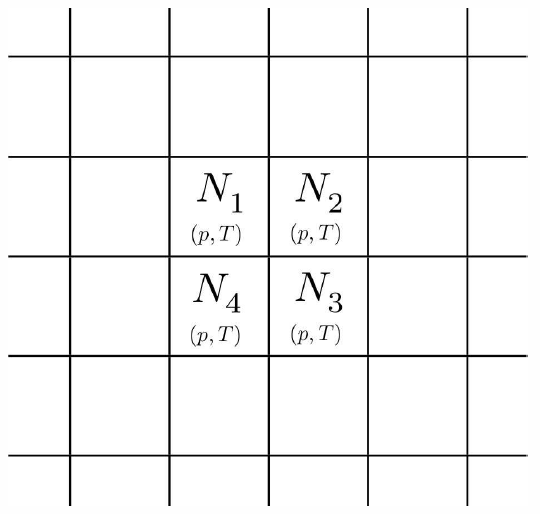
Now let us imagine removing all the barriers separating the different gases and letting the particles mix thoroughly. The result is that each component gas occupies the full volume V, so the entropy is S∗mixed=∑aS∗a=∑a[N∗akBln(V/N∗a)+N∗aϕ∗a(T)] . Thus, the entropy of mixing is ΔS∗mix=S∗mixed−S∗unmixed=∑aN∗akBln(V/V∗a)=−NkB∑ax∗alnx∗a , where x∗a=NaN=VaV is the fraction of species a. Note that ΔS∗mix≥0.
What if all the components were initially identical? It seems absurd that the entropy should increase simply by removing some invisible barriers. This is again the Gibbs paradox. In this case, the resolution of the paradox is to note that the sum in the expression for S∗mixed is a sum over distinct species. Hence if the particles are all identical, we have S∗mixed=NkBln(V/N)+Nϕ(T)=S∗unmixed, hence ΔS∗mix=0.
Entropy and combinatorics
As we shall learn when we study statistical mechanics, the entropy may be interpreted in terms of the number of ways W(E,V,N) a system at fixed energy and volume can arrange itself. One has S(E,V,N)=kBlnW(E,V,N) . Consider a system consisting of σ different species of particles. Now let it be that for each species label a, N∗a particles of that species are confined among Q∗a little boxes such that at most one particle can fit in a box (see Fig. [Smix]). How many ways W are there to configure N identical particles among Q boxes? Clearly W={Q\choose N}={Q!\over N! \, (Q-N)!}\ . Were the particles distinct, we’d have W\ns_{distinct}={Q!\over(Q-N)!}, which is N! times greater. This is because permuting distinct particles results in a different configuration, and there are N! ways to permute N particles.
The entropy for species a is then S\ns_a=\kB\ln W\ns_a=\kB\ln\!\Big({Q\ns_a\atop N\ns_a}\Big). We then use Stirling’s approximation, \ln(K!) = K\ln K - K + \half\ln K + \half\ln(2\pi) + \CO(K^{-1})\ , which is an asymptotic expansion valid for K\gg 1. One then finds for Q,N\gg 1, with x=N/Q\in [0,1], \begin{aligned} \ln {Q\choose N} &= \Big( Q\ln Q - Q \Big) - \Big(xQ\ln(xQ)-xQ\Big) - \Big((1-x)Q\ln\big((1-x)Q\big)-(1-x)Q\Big) \nonumber \\ &=-Q\Big[x\ln x + (1-x)\ln(1-x)\Big]\ .\end{aligned} This is valid up to terms of order Q in Stirling’s expansion. Since \ln Q \ll Q, the next term is small and we are safe to stop here. Summing up the contributions from all the species, we get S\ns_{unmixed} = \kB\sum_{a=1}^\sigma\ln W\ns_a = - \kB\sum_{a=1}^\sigma Q\ns_a \Big[x\ns_a\ln x\ns_a + (1-x\ns_a)\ln(1-x\ns_a)\Big]\ , where x\ns_a=N\ns_a/Q\ns_a is the initial dimensionless density of species a.
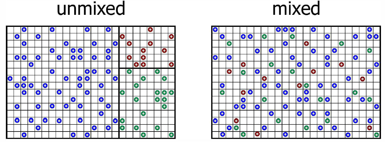
Now let’s remove all the partitions between the different species so that each of the particles is free to explore all of the boxes. There are Q=\sum_a Q\ns_a boxes in all. The total number of ways of placing N\ns_1 particles of species a=1 through N\ns_\sigma particles of species \sigma is W\ns_{mixed}={Q!\over N\ns_0! \, N\ns_1! \cdots N\ns_\sigma!}\ , where N\ns_0=Q-\sum_{a=1}^\sigma N\ns_a is the number of vacant boxes. Again using Stirling’s rule, we find S\ns_{mixed}=-\kB\,Q \sum_{a=0}^\sigma {\widetilde x}\ns_a \ln {\widetilde x}\ns_a\ , where {\widetilde x}\ns_a=N\ns_a/Q is the fraction of all boxes containing a particle of species a, and N\ns_0 is the number of empty boxes. Note that {\widetilde x}\ns_a={N\ns_a\over Q}={N\ns_a\over Q\ns_a}\cdot{Q\ns_a\over Q}=x\ns_a \, f\ns_a\ , where f\ns_a\equiv Q\ns_a/Q. Note that \sum_{a=1}^\sigma f\ns_a=1.
Let’s assume all the densities are initially the same, so x\ns_a=x\forall a, so {\widetilde x}\ns_a=x\,f\ns_a. In this case, f\ns_a={Q\ns_a\over Q}={N\ns_a\over N} is the fraction of species a among all the particles. We then have {\widetilde x}\ns_0=1-x, and \begin{split} S\ns_{mixed}&=-\kB\, Q\sum_{a=1}^\sigma x f\ns_a\ln (x f\ns_a) - \kB \,Q\,{\widetilde x}\ns_0\ln{\widetilde x}\ns_0\\ &=-\kB \,Q \Big[x\ln x + (1-x)\ln(1-x)\Big] - \kB\,x\,Q\sum_{a=1}^\sigma f\ns_a\ln f\ns_a\ . \end{split} Thus, the entropy of mixing is \RDelta S\ns_{mix}=-N\kB\sum_{a=1}^\sigma f\ns_a\ln f\ns_a \ , where N=\sum_{a=1}^\sigma N\ns_a is the total number of particles among all species (excluding vacancies) and f\ns_a=N\ns_a/(N+N\ns_0) is the fraction of all boxes occupied by species a.
Weak solutions and osmotic pressure
Suppose one of the species is much more plentiful than all the others, and label it with a=0. We will call this the solvent. The entropy of mixing is then \RDelta S\ns_{mix}=-\kB\Bigg[N\ns_0\ln\!\bigg({N\ns_0\over N\ns_0+N'}\bigg) + \sum_{a=1}^\sigma N\ns_a\ln\!\bigg({N\ns_a\over N\ns_0+N'}\bigg)\Bigg]\ , where N'=\sum_{a=1}^\sigma N\ns_a is the total number of solvent molecules, summed over all species. We assume the solution is weak, which means N\ns_a\le N'\ll N\ns_0. Expanding in powers of N'/N\ns_0 and N\ns_a/N\ns_0, we find \RDelta S\ns_{mix}=-\kB\sum_{a=1}^\sigma\Bigg[N\ns_a\ln\!\bigg({N\ns_a\over N\ns_0}\bigg) -N\ns_a\Bigg] + \CO\big({N'}^2/N\ns_0\big)\ . \label{smixweak}
Consider now a solution consisting of N\ns_0 molecules of a solvent and N\ns_a molecules of species a of solute, where a=1,\ldots,\sigma. We begin by expanding the Gibbs free energy G(T,p,N\ns_0,N\ns_1,\ldots,N\ns_\sigma), where there are \sigma species of solutes, as a power series in the small quantities N\ns_a. We have \begin{split} G\big(T,p,N\ns_0,\{N\ns_a\}\big)&=N\ns_0\, g\ns_0(T,p) + \kT\sum_a N\ns_a \ln\!\bigg({N\ns_a\over e N\ns_0}\bigg)\\ &\qquad\qquad + \sum_a N\ns_a\,\psi\ns_a(T,p) + {1\over 2N\ns_0}\sum_{a,b} A\ns_{ab}(T,p)\,N\ns_a \,N\ns_b\ . \end{split} The first term on the RHS corresponds to the Gibbs free energy of the solvent. The second term is due to the entropy of mixing. The third term is the contribution to the total free energy from the individual species. Note the factor of e in the denominator inside the logarithm, which accounts for the second term in the brackets on the RHS of Equation \ref{smixweak}. The last term is due to interactions between the species; it is truncated at second order in the solute numbers.
The chemical potential for the solvent is \mu\ns_0(T,p)={\pz G\over\pz N\ns_0}= g\ns_0(T,p) - \kT\sum_a x\ns_a -\half\sum_{a,b} A\ns_{ab}(T,p)\,x\ns_a\, x\ns_b\ , and the chemical potential for species a is \mu\ns_a(T,p)={\pz G\over\pz N\ns_a}=\kT\ln x\ns_a + \psi\ns_a(T,p) + \sum_b A\ns_{ab}(T,p)\,x\ns_b\ , where x\ns_a=N\ns_a/N\ns_0 is the concentrations of solute species a. By assumption, the last term on the RHS of each of these equations is small, since N\ns_{solute}\ll N\ns_0, where N\ns_{solute}=\sum_{a=1}^\sigma N\ns_a is the total number of solute molecules. To lowest order, then, we have \begin{aligned} \mu\ns_0(T,p)&= g\ns_0(T,p) - x\,\kT\\ \mu\ns_a(T,p)&=\kT\ln x\ns_a + \psi\ns_a(T,p) \ ,\end{aligned} where x=\sum_a x\ns_a is the total solute concentration.
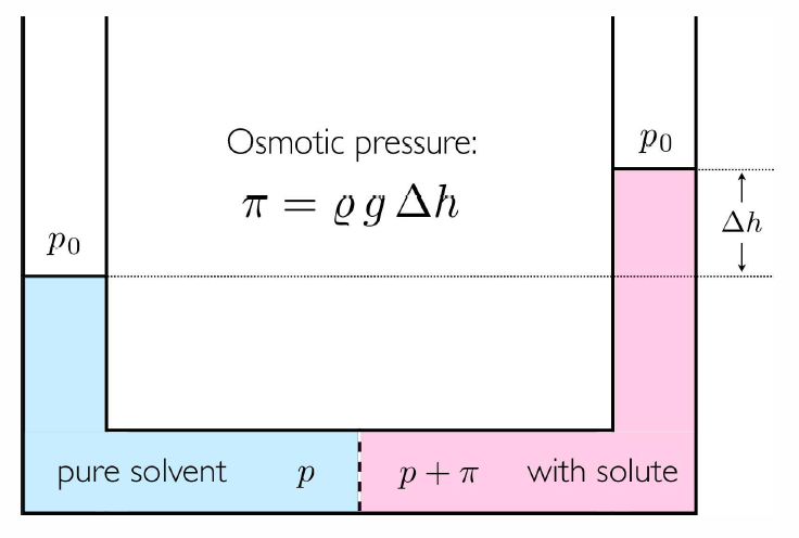
If we add sugar to a solution confined by a semipermeable membrane19, the pressure increases! To see why, consider a situation where a rigid semipermeable membrane separates a solution (solvent plus solutes) from a pure solvent. There is energy exchange through the membrane, so the temperature is T throughout. There is no volume exchange, however: dV=dV'=0, hence the pressure need not be the same. Since the membrane is permeable to the solvent, we have that the chemical potential \mu\ns_0 is the same on each side. This means
g_0\left(T, p_{\mathrm{R}}\right)-x k_{\mathrm{B}} T=g_0\left(T, p_{\mathrm{L}}\right)
where p_{\mathrm{L}, \mathrm{R}} is the pressure on the left and right sides of the membrane, and x=N / N_0 is again the total solute concentration. This equation once again tells us that the pressure p cannot be the same on both sides of the membrane. If the pressure difference is small, we can expand in powers of the osmotic pressure, \pi \equiv p_{\mathrm{R}}-p_{\mathrm{L}}, and we find
\pi=x k_{\mathrm{B}} T /\left(\frac{\partial \mu_0}{\partial p}\right)_T
\pi= x\,\kT\bigg/\pabc{\mu\ns_0}{p}{T}\ . But a Maxwell relation (§9) guarantees \pabc{\mu}{p}{T,N}=\pabc{V}{N}{T,p} = v(T,p)/\NA\ , where v(T,p) is the molar volume of the solvent. \pi v=xR T\ , which looks very much like the ideal gas law, even though we are talking about dense (but ‘weak’) solutions! The resulting pressure has a demonstrable effect, as sketched in Fig. [osmotic]. Consider a solution containing \nu moles of sucrose (\RC\ns_{12}\RH\ns_{22}\RO\ns_{11}) per kilogram (55.52\,{mol}) of water at 30^\circ\,\RC. We find \pi=2.5\,{atm} when \nu=0.1.
One might worry about the expansion in powers of \pi when \pi is much larger than the ambient pressure. But in fact the next term in the expansion is smaller than the first term by a factor of \pi\kappa\ns_T, where \kappa\ns_T is the isothermal compressibility. For water one has \kappa\ns_T\approx 4.4\times 10^{-5}\,({atm})^{-1}, hence we can safely ignore the higher order terms in the Taylor expansion.
Effect of impurities on boiling and freezing points
Along the coexistence curve separating liquid and vapor phases, the chemical potentials of the two phases are identical:
\mu_{\mathrm{L}}^0(T, p)=\mu_{\mathrm{V}}^0(T, p)
Here we write \mu^0 for \mu to emphasize that we are talking about a phase with no impurities present. This equation provides a single constraint on the two variables T and p, hence one can, in principle, solve to obtain T=T_0^*(p), which is the equation of the liquid-vapor coexistence curve in the (T, p) plane. Now suppose there is a solute present in the liquid. We then have
\mu_{\mathrm{L}}(T, p, x)=\mu_{\mathrm{L}}^0(T, p)-x k_{\mathrm{B}} T
where x is the dimensionless solute concentration, summed over all species. The condition for liquid-vapor coexistence now becomes
\mu^0_\ssr{L}(T,p)-x\kT=\mu^0_\ssr{V}(T,p)\ .
\mu_{\mathrm{L}}^0(T, p)-x k_{\mathrm{B}} T=\mu_{\mathrm{V}}^0(T, p) .
This will lead to a shift in the boiling temperature at fixed p. Assuming this shift is small, let us expand to lowest order in \left(T-T_0^*(p)\right), writing
\mu_{\mathrm{L}}^0\left(T_0^*, p\right)+\left(\frac{\partial \mu_{\mathrm{L}}^0}{\partial T}\right)_p\left(T-T_0^*\right)-x k_{\mathrm{B}} T=\mu_{\mathrm{v}}^0\left(T_0^*, p\right)+\left(\frac{\partial \mu_{\mathrm{v}}^0}{\partial T}\right)_p\left(T-T_0^*\right)
Note that
\left(\frac{\partial \mu}{\partial T}\right)_{p, N}=-\left(\frac{\partial S}{\partial N}\right)_{T, p}
from a Maxwell relation deriving from exactness of d G. Since S is extensive, we can write S= \left(N / N_{\mathrm{A}}\right) s(T, p), where s(T, p) is the molar entropy. Solving for T, we obtain
T^*(p, x)=T_0^*(p)+\frac{x R\left[T_0^*(p)\right]^2}{\ell_{\mathrm{v}}(p)}
where \ell_{\mathrm{v}}=T_0^* \cdot\left(s_{\mathrm{V}}-s_{\mathrm{L}}\right) is the latent heat of the liquid-vapor transition { }^{20}. The shift \Delta T^*=T^*-T_0^* is called the boiling point elevation.
As an example, consider seawater, which contains approximately 35 g of dissolved \mathrm{Na}^{+} \mathrm{Cl}^{-}per kilogram of \mathrm{H}_2 \mathrm{O}. The atomic masses of Na and Cl are 23.0 and 35.4 , respectively, hence the total ionic concentration in seawater (neglecting everything but sodium and chlorine) is given by
x=\frac{2 \cdot 35}{23.0+35.4} / \frac{1000}{18} \approx 0.022
| Latent Heat | Melting | Latent Heat of | Boiling | |
|---|---|---|---|---|
| Substance | of Fusion {\tilde \ell}_\Rf | Point | Vaporization {\tilde \ell}_\Rv | Point |
| \RJ/\Rg | {}^\circ\RC | \RJ/\Rg | {}^\circ\RC | |
| \RC\ns_2\RH\ns_5\RO\RH | 108 | -114 | 855 | 78.3 |
| \RN\RH\ns_3 | 339 | -75 | 1369 | -33.34 |
| \RC\RO\ns_2 | 184 | -57 | 574 | -78 |
| He | – | – | 21 | -268.93 |
| H | 58 | -259 | 455 | -253 |
| Pb | 24.5 | 372.3 | 871 | 1750 |
| \RN\ns_2 | 25.7 | -210 | 200 | -196 |
| \RO\ns_2 | 13.9 | -219 | 213 | -183 |
| \RH\ns_2\RO | 334 | 0 | 2270 | 100 |
The latent heat of vaporization of \RH\ns_2\RO at atmospheric pressure is \ell=40.7\,{kJ}/{mol}, hence \RDelta T^*={(0.022)(8.3\,\RJ/{mol}\,\RK) (373\,\RK)^2\over 4.1\times 10^4 \,\RJ/{mol}}\approx 0.6\,\RK\ . Put another way, the boiling point elevation of \RH\ns_2\RO at atmospheric pressure is about 0.28^\circ\RC per percent solute. We can express this as \RDelta T^*=Km, where the molality m is the number of moles of solute per kilogram of solvent. For \RH\ns_2\RO, we find K=0.51^\circ\RC\,{kg}/{mol}.
Similar considerations apply at the freezing point, when we equate the chemical potential of the solvent plus solute to that of the pure solid. The latent heat of fusion for \mathrm{H}_2 \mathrm{O} is about \ell_{\mathrm{f}}=T_{\mathrm{f}}^0 \cdot\left(s_{\text {LIQUID }}-s_{\text {SOLID }}\right)= 6.01 \mathrm{~kJ} / \mathrm{mol}^{21} We thus predict a freezing point depression of \Delta T^*=-x R\left[T_0^*\right]^2 / \ell_{\mathrm{f}}=1.03^{\circ} \mathrm{C} \cdot x[\%]. This can be expressed once again as \Delta T^*=-K m, with K=1.86^{\circ} \mathrm{C} \mathrm{kg} / \mathrm{mol}^{22}.
Binary solutions
Consider a binary solution, and write the Gibbs free energy G(T,p,N\ns_\SA,N\ns_\SB) as \begin{split} G(T,p,N\ns_\SA,N\ns_\SB)&=N\ns_\SA\,\mu^0_\SA(T,p) + N\ns_\SB\,\mu^0_\SB(T,p) + N\ns_\SA \kT\,\ln\bigg({N\ns_\SA\over N\ns_\SA+N\ns_\SB}\bigg)\\ &\qquad + N\ns_\SB\, \kT\,\ln\!\bigg({N\ns_\SB\over N\ns_\SA+N\ns_\SB}\bigg) + \lambda\,{N\ns_\SA N\ns_\SB\over \> N\ns_\SA+N\ns_\SB\>}\ . \end{split} The first four terms on the RHS represent the free energy of the individual component fluids and the entropy of mixing. The last term is an interaction contribution. With \lambda>0, the interaction term prefers that the system be either fully \SA or fully \SB. The entropy contribution prefers a mixture, so there is a competition. What is the stable thermodynamic state?
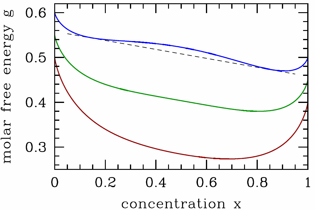
[binary] : Gibbs free energy per particle for a binary solution as a function of concentration x=x_{\mathrm{B}} of the B species (pure A at the left end x=0; pure B at the right end x=1 ), in units of the interaction parameter \lambda. Dark red curve: T=0.65 \lambda / k_{\mathrm{B}}>T_{\mathrm{c}}; green curve: T=\lambda / 2 k_{\mathrm{B}}=T_{\mathrm{c}}; blue curve: T=0.40 \lambda / k_{\mathrm{B}}<T_{\mathrm{c}}. We have chosen \mu_{\mathrm{A}}^0=0.60 \lambda-0.50 k_{\mathrm{B}} T and \mu_{\mathrm{B}}^0=0.50 \lambda-0.50 k_{\mathrm{B}} T. Note that the free energy g(T, p, x) is not convex in x for T<T_{\mathrm{c}}, indicating an instability and necessitating a Maxwell construction.
It is useful to write the Gibbs free energy per particle, g(T,p,x)=G/(N\ns_\SA+N\ns_\SB), in terms of T, p, and the concentration x\equiv x\ns_\SB=N\ns_\SB/(N\ns_\SA+N\ns_\SB) of species B (hence x\ns_\SA=1-x is the concentration of species A). Then g(T,p,x)=(1-x)\,\mu^0_\SA+x\,\mu^0_\SB+ \kT\Big[x\ln x + (1-x)\ln(1-x)\Big] + \lambda\, x\,(1-x)\ . In order for the system to be stable against phase separation into relatively \SA-rich and \SB-rich regions, we must have that g(T,p,x) be a convex function of x. Our first check should be for a local instability, spinodal decomposition. We have {\pz g\over\pz x}=\mu^0_\SB-\mu^0_\SA + \kT\,\ln\bigg({x\over 1-x}\bigg) + \lambda\,(1-2x) \label{gpmax} and {\pz^2\!g\over\pz x^2}={\kT\over x} + {\kT\over 1-x} - 2\lambda \ . The spinodal is given by the solution to the equation {\pz^2\!g\over\pz x^2}=0, which is T^*(x)={2\lambda\over \kB}\,x\,(1-x)\ . \label{TSPINO} Since x\,(1-x) achieves its maximum value of \frac{1}{4} at x=\half, we have T^*\le \kB/2\lambda.
In Fig. [bing] we sketch the free energy g(T,p,x) versus x for three representative temperatures. For T>\lambda/2\kB, the free energy is everywhere convex in \lambda. When T<\lambda/2\kB, there free energy resembles the blue curve in Fig. [bing], and the system is unstable to phase separation. The two phases are said to be immiscible, or, equivalently, there exists a solubility gap. To determine the coexistence curve, we perform a Maxwell construction, writing {g(x\ns_2)-g(x\ns_1)\over x\ns_2-x\ns_1}={\pz g\over\pz x}\bigg|\nd_{x\ns_1}={\pz g\over\pz x}\bigg|\nd_{x\ns_2}\ . \label{binmax} Here, x\ns_1 and x\ns_2 are the boundaries of the two phase region. These equations admit a symmetry of x\leftrightarrow 1-x, hence we can set x=x\ns_1 and x\ns_2=1-x. We find g(1-x)-g(x)=(1-2x)\,\big(\mu_\SB^0-\mu_\SA^0\big)\ , and invoking eqns. [binmax] and [gpmax] we obtain the solution T\ns_{coex}(x)={\lambda\over \kB}\cdot{1-2x\over \ \ln\big({1-x\over x}\big)\>}\ . \label{TCOEX}
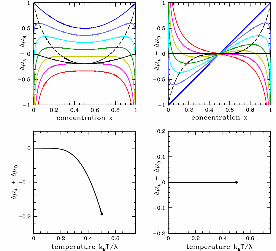
[binmupd] Upper panels: chemical potential shifts \RDelta\mu_\pm=\RDelta\mu_\SA\pm\RDelta\mu_\SB versus concentration x=x_\SB. The dashed black line is the spinodal, and the solid black line the coexistence boundary. Temperatures range from T=0 (dark blue) to T=0.6\,\lambda/k_\ssr{B} (red) in units of 0.1\,\lambda/k_\ssr{B}. Lower panels: phase diagram in the (T,\RDelta\mu_\pm) planes. The black dot is the critical point.
The phase diagram for the binary system is shown in Fig. [binary]. For T<T^*(x), the system is unstable, and spinodal decomposition occurs. For T^*(x) < T < T\ns_{coex}(x), the system is metastable, just like the van der Waals gas in its corresponding regime. Real binary solutions behave qualitatively like the model discussed here, although the coexistence curve is generally not symmetric under x\leftrightarrow 1-x, and the single phase region extends down to low temperatures for x\approx 0 and x\approx 1. If \lambda itself is temperature-dependent, there can be multiple solutions to eqns. [TSPINO] and [TCOEX]. For example, one could take \lambda(T)={\lambda\ns_0\,T^2\over T^2 + T_0^2}\ . In this case, \kT > \lambda at both high and low temperatures, and we expect the single phase region to be reentrant. Such a phenomenon occurs in water-nicotine mixtures, for example.
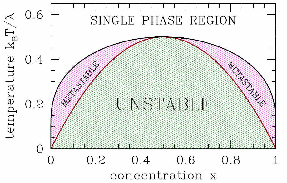
[binary] Phase diagram for the binary system. The black curve is the coexistence curve, and the dark red curve is the spinodal. A-rich material is to the left and B-rich to the right.
It is instructive to consider the phase diagram in the (T,\mu) plane. We define the chemical potential shifts, \begin{aligned} \RDelta\mu\ns_\SA&\equiv\mu\ns_\SA-\mu^0_\SA=\kT\ln(1-x)+\lambda\,x^2 \\ \RDelta\mu\ns_\SB&\equiv\mu\ns_\SB-\mu^0_\SB=\kT\ln x+\lambda\,(1-x)^2\ ,\end{aligned} and their sum and difference, \RDelta\mu\ns_\pm\equiv\RDelta\mu\ns_\SA\pm \RDelta\mu\ns_\SB. From the Gibbs-Duhem relation, we know that we can write \mu\ns_\SB as a function of T, p, and \mu\ns_\SA. Alternately, we could write \RDelta\mu\ns_\pm in terms of T, p, and \RDelta\mu\ns_\mp, so we can choose which among \RDelta\mu\ns_+ and \RDelta\mu\ns_- we wish to use in our phase diagram. The results are plotted in Fig. [binmupd]. It is perhaps easiest to understand the phase diagram in the (T,\RDelta\mu\ns_-) plane. At low temperatures, below T=T\ns_\Rc=\lambda/2\kB, there is a first order phase transition at \RDelta\mu\ns_-=0. For T<T\ns_\Rc=\lambda/2\kB and \RDelta\mu\ns_-=0^+, infinitesimally positive, the system is in the \SA-rich phase, but for \RDelta\mu\ns_-=0^-, infinitesimally negative, it is \SB-rich. The concentration x=x\ns_\SB changes discontinuously across the phase boundary. The critical point lies at (T,\RDelta\mu\ns_-)=(\lambda/2\kB\,,\,0).
If we choose N=N\ns_\SA+N\ns_\SB to be the extensive variable, then fixing N means dN\ns_\SA+ dN\ns_\SB=0. So st fixed T and p, dG\big|\ns_{T,p}=\mu\ns_\SA\,dN\ns_\SA + \mu\ns_\SB\,dN\ns_\SB \qquad \Rightarrow \qquad dg\big|\nd_{T,p}=-\RDelta\mu\ns_-\,dx\ . Since \RDelta\mu\ns_-(x,T)=\vphi(x,T)-\vphi(1-x,T)=-\RDelta\mu\ns_-(1-x,T), where \vphi(x,T) = \lambda x - \kT\ln x, we have that the coexistence boundary in the (x,\RDelta\ns_-) plane is simply the line \RDelta\mu\ns_-=0, because \int\limits_x^{1-x}\!\!\! dx'\,\RDelta\mu\ns_-(x',T)=0.
Note also that there is no two-phase region in the (T,\RDelta\mu) plane; the phase boundary in this plane is a curve which terminates at a critical point. As we saw in §12, the same situation pertains in single component (p,v,T) systems. That is, the phase diagram in the (p,v) or (T,v) plane contains two-phase regions, but in the (p,T) plane the boundaries between phases are one-dimensional curves. Any two-phase behavior is confined to these curves, where the thermodynamic potentials are singular.
The phase separation can be seen in a number of systems. A popular example involves mixtures of water and ouzo or other anise-based liqueurs, such as arak and absinthe. Starting with the pure liqueur (x=1), and at a temperature below the coexistence curve maximum, the concentration is diluted by adding water. Follow along on Fig. [binary] by starting at the point (x=1\,,\,\kT/\lambda=0.4) and move to the left. Eventually, one hits the boundary of the two-phase region. At this point, the mixture turns milky, due to the formation of large droplets of the pure phases on either side of coexistence region which scatter light, a process known as spontaneous emulsification23. As one continues to dilute the solution with more water, eventually one passes all the way through the coexistence region, at which point the solution becomes clear once again, and described as a single phase.
What happens if \lambda<0\>? In this case, both the entropy and the interaction energy prefer a mixed phase, and there is no instability to phase separation. The two fluids are said to be completely miscible. An example would be benzene, \RC\ns_6\RH\ns_6, and toluene, \RC\ns_7\RH\ns_8 ( \RC\ns_6\RH\ns_5{CH}\ns_3). The phase diagram would be blank, with no phase boundaries below the boiling transition, because the fluid could exist as a mixture in any proportion.
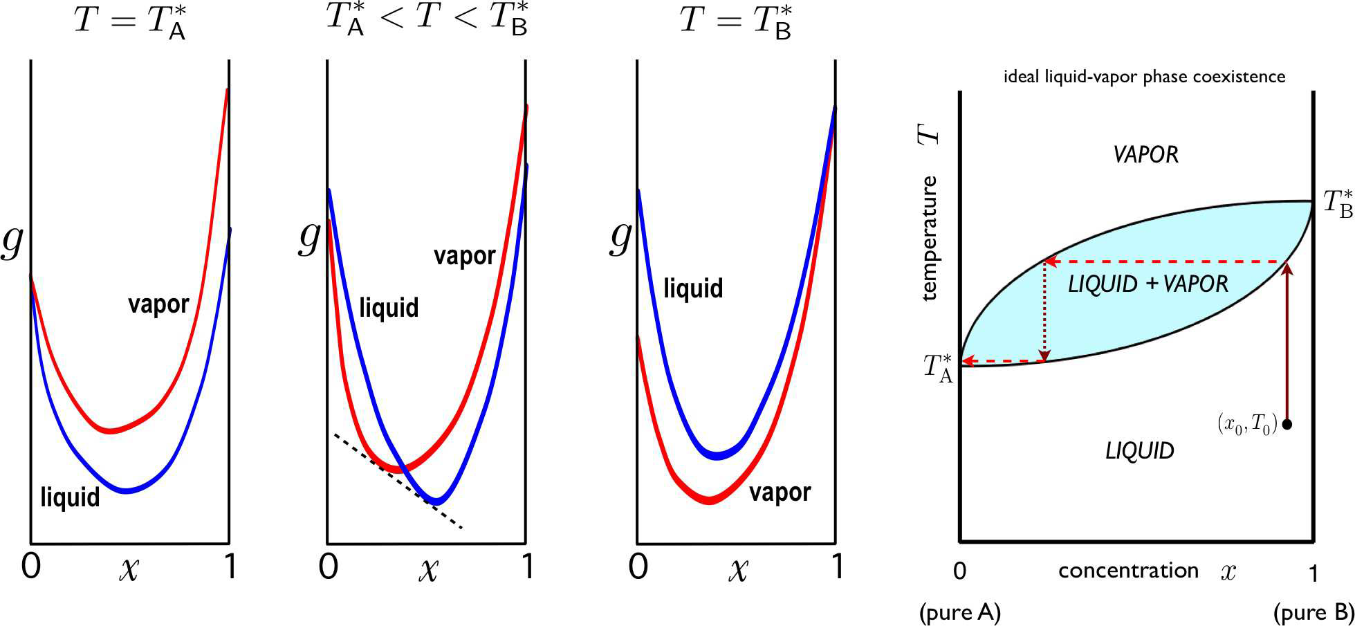
Figure [LVcoex] Gibbs free energy per particle g for an ideal binary solution for temperatures T\in [T^*_\SA,T^*_\SB]. The Maxwell construction is shown for the case T^*_\SA < T < T^*_\SB. Right: phase diagram, showing two-phase region and distillation sequence in (x,T) space.
Any fluid will eventually boil if the temperature is raised sufficiently high. Let us assume that the boiling points of our A and B fluids are T_{\mathrm{A}, \mathrm{B}}^*, and without loss of generality let us take T_{\mathrm{A}}^*<T_{\mathrm{B}}^* at some given fixed pressure { }^{24}. This means \mu_{\mathrm{A}}^{\mathrm{L}}\left(T_{\mathrm{A}}^*, p\right)=\mu_{\mathrm{A}}^{\mathrm{V}}\left(T_{\mathrm{A}}^*, p\right) and \mu_{\mathrm{B}}^{\mathrm{L}}\left(T_{\mathrm{B}}^*, p\right)=\mu_{\mathrm{B}}^{\mathrm{V}}\left(T_{\mathrm{B}}^*, p\right). What happens to the mixture
mixture? We begin by writing the free energies of the mixed liquid and mixed vapor phases as
\begin{array}{l} g_{\mathrm{L}}(T, p, x)=(1-x) \mu_{\mathrm{A}}^{\mathrm{L}}(T, p)+x \mu_{\mathrm{B}}^{\mathrm{L}}(T, p)+k_{\mathrm{B}} T[x \ln x+(1-x) \ln (1-x)]+\lambda_{\mathrm{L}} x(1-x) \\ g_{\mathrm{V}}(T, p, x)=(1-x) \mu_{\mathrm{A}}^{\mathrm{V}}(T, p)+x \mu_{\mathrm{B}}^{\mathrm{V}}(T, p)+k_{\mathrm{B}} T[x \ln x+(1-x) \ln (1-x)]+\lambda_{\mathrm{V}} x(1-x) \end{array}
Typically \lambda_{\mathrm{V}} \approx 0. Consider these two free energies as functions of the concentration x, at fixed T and p. If the curves never cross, and g_{\mathrm{L}}(x)<g_{\mathrm{V}}(x) for all x \in[0,1], then the liquid is always the state of lowest free energy. This is the situation in the first panel of Fig. 2.37. Similarly, if g_{\mathrm{V}}(x)<g_{\mathrm{L}}(x) over this range, then the mixture is in the vapor phase throughout. What happens if the two curves cross at some value of x ? This situation is depicted in the second panel of Fig. 2.37. In this case, there is always a Maxwell construction which lowers the free energy throughout some range of concentration, i.e. the system undergoes phase separation.
In an ideal fluid, we have \lambda_{\mathrm{L}}=\lambda_{\mathrm{V}}=0, and setting g_{\mathrm{L}}=g_{\mathrm{V}} requires
(1-x) \Delta \mu_{\mathrm{A}}(T, p)+x \Delta \mu_{\mathrm{B}}(T, p)=0
where \Delta \mu_{\mathrm{A} / \mathrm{B}}(T, p)=\mu_{\mathrm{A} / \mathrm{B}}^{\mathrm{L}}(T, p)-\mu_{\mathrm{A} / \mathrm{B}}^{\mathrm{V}}(T, p). Expanding the chemical potential about a given temperature T^*,
\mu(T, p)=\mu\left(T^*, p\right)-s\left(T^*, p\right)\left(T-T^*\right)-\frac{c_p\left(T^*, p\right)}{2 T}\left(T-T^*\right)^2+\ldots
where we have used \left(\frac{\partial \mu}{\partial T}\right)_{p, N}=-\left(\frac{\partial S}{\partial N}\right)_{T, p}=-s(T, p), the entropy per particle, and \left(\frac{\partial s}{\partial T}\right)_{p, N}=c_p / T.
 Figure
Thus, expanding \Delta \mu_{\mathrm{A} / \mathrm{B}} about T_{\mathrm{A} / \mathrm{B}}^*, we have
\begin{array}{l} \Delta \mu_{\mathrm{A}} \equiv \mu_{\mathrm{A}}^{\mathrm{L}}-\mu_{\mathrm{A}}^{\mathrm{V}}=\left(s_{\mathrm{A}}^{\mathrm{V}}-s_{\mathrm{A}}^{\mathrm{L}}\right)\left(T-T_{\mathrm{A}}^*\right)+\frac{c_{p \mathrm{~A}}^{\mathrm{V}}-c_{p \mathrm{~A}}^{\mathrm{L}}}{2 T_{\mathrm{A}}^*}\left(T-T_{\mathrm{A}}^*\right)^2+\ldots \\ \Delta \mu_{\mathrm{B}} \equiv \mu_{\mathrm{B}}^{\mathrm{L}}-\mu_{\mathrm{B}}^{\mathrm{V}}=\left(s_{\mathrm{B}}^{\mathrm{V}}-s_{\mathrm{B}}^{\mathrm{L}}\right)\left(T-T_{\mathrm{B}}^*\right)+\frac{c_{p \mathrm{~B}}^{\mathrm{V}}-c_{p \mathrm{~B}}^{\mathrm{L}}}{2 T_{\mathrm{B}}^*}\left(T-T_{\mathrm{B}}^*\right)^2+\ldots \end{array}
We assume s_{\mathrm{A} / \mathrm{B}}^{\mathrm{V}}>s_{\mathrm{A} / \mathrm{B}}^{\mathrm{L}}, i.e. the vapor phase has greater entropy per particle. Thus, \Delta \mu_{\mathrm{A} / \mathrm{B}}(T) changes sign from negative to positive as T rises through T_{\mathrm{A} / \mathrm{B}}^*. If we assume that these are the only sign changes for \Delta \mu_{\mathrm{A} / \mathrm{B}}(T) at fixed p, then eqn. [muABbin] can only be solved for T \in\left[T_{\mathrm{A}}^*, T_{\mathrm{B}}^*\right]. This immediately leads to the phase diagram in the rightmost panel of Fig. [LVcoex].
According to the Gibbs phase rule, with \sigma=2, two-phase equilibrium (\varphi=2) occurs along a subspace of dimension d\ns_\ssr{PE}=2+\sigma-\varphi=2. Thus, if we fix the pressure p and the concentration x=x\subB, liquid-gas equilibrium occurs at a particular temperature T^*, known as the boiling point. Since the liquid and the vapor with which it is in equilibrium at T^* may have different composition, different values of x, one may distill the mixture to separate the two pure substances, as follows. First, given a liquid mixture of \SA and \SB, we bring it to boiling, as shown in the rightmost panel of Fig. [LVcoex]. The vapor is at a different concentration x than the liquid (a lower value of x if the boiling point of pure \SA is less than that of pure \SB, as shown). If we collect the vapor, the remaining fluid is at a higher value of x. The collected vapor is then captured and then condensed, forming a liquid at the lower x value. This is then brought to a boil, and the resulting vapor is drawn off and condensed, etc The result is a purified \SA state. The remaining liquid is then at a higher \SB concentration. By repeated boiling and condensation, \SA and \SB can be separated. For liquid-vapor transitions, the upper curve, representing the lowest temperature at a given concentration for which the mixture is a homogeneous vapor, is called the dew point curve. The lower curve, representing the highest temperature at a given concentration for which the mixture is a homogeneous liquid, is called the bubble point curve. The same phase diagram applies to liquid-solid mixtures where both phases are completely miscible. In that case, the upper curve is called the liquidus, and the lower curve the solidus.
When a homogeneous liquid or vapor at concentration x is heated or cooled to a temperature T such that (x, T) lies within the two-phase region, the mixture phase separates into the the two end components \left(x_{\mathrm{L}}^*, T\right) and \left(x_{\mathrm{V}}^*, T\right), which lie on opposite sides of the boundary of the two-phase region, at the same temperature. The locus of points at constant T joining these two points is called the tie line. To determine how much of each of these two homogeneous phases separates out, we use particle number conservation. If \eta_{\mathrm{L}, \mathrm{V}} is the fraction of the homogeneous liquid and homogeneous vapor phases present, then \eta_{\mathrm{L}} x_{\mathrm{L}}^*+\eta_{\mathrm{V}} x_{\mathrm{V}}^*=x, which says \eta_{\mathrm{L}}=\left(x-x_{\mathrm{V}}^*\right) /\left(x_{\mathrm{L}}^*-x_{\mathrm{V}}^*\right) and \eta_{\mathrm{V}}=\left(x-x_{\mathrm{L}}^*\right) /\left(x_{\mathrm{V}}^*-x_{\mathrm{L}}^*\right). This is known as the lever rule.
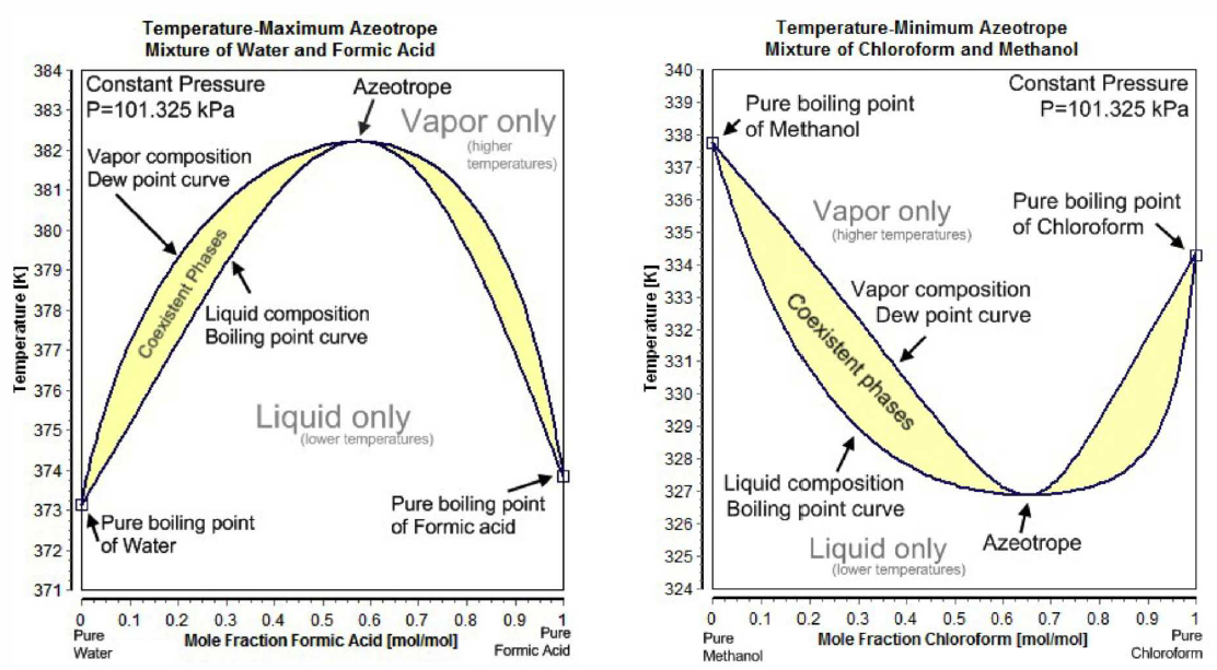
For many binary mixtures, the boiling point curve is as shown in Fig. [FAZEO]. Such cases are called azeotropes. For negative azeotropes, the maximum of the boiling curve lies above both T_{\mathrm{A}, \mathrm{B}}^*. The free energy curves for this case are shown in panel (b) of Fig. [FAZZ]. For x<x^*, where x^* is the azeotropic composition, one can distill A but not B. Similarly, for x>x^* one can distill B but not A . The situation is different for positive azeotropes, where the minimum of the boiling curve lies below both T_{\mathrm{A}, \mathrm{B}}^*, corresponding to the free energy curves in panel (c) of Fig. [FAZZ]. In this case, distillation (i.e. condensing and reboiling the collected vapor) from either side of x^* results in the azeotrope. One can of course collect the fluid instead of the vapor. In general, for both positive and negative azeotropes, starting from a given concentration x, one can only arrive at pure A plus azeotrope (if x<x^* ) or pure B plus azeotrope (if \left.x>x^*\right). Ethanol \left(\mathrm{C}_2 \mathrm{H}_5 \mathrm{OH}\right) and water \left(\mathrm{H}_2 \mathrm{O}\right) form a positive azeotrope which is 95.6 \% ethanol and 4.4 \% water by weight. The individual boiling points are T_{\mathrm{C}_2 \mathrm{H}_5 \mathrm{OH}}^*=78.4^{\circ} \mathrm{C}, T_{\mathrm{H}_2 \mathrm{O}}^*=100^{\circ} \mathrm{C}, while the azeotrope boils at T_{\mathrm{AZ}}^*=78.2^{\circ} \mathrm{C}. No amount of distillation of this mixture can purify ethanol beyond the 95.6 \% level. To go beyond this level of purity, one must resort to azeotropic distillation, which involves introducing another component, such as benzene (or a less carcinogenic additive), which alters the molecular interactions.
To model the azeotrope system, we need to take \lambda_{\mathrm{L}} \neq 0, in which case one can find two solutions to the energy crossing condition g_{\mathrm{V}}(x)=g_{\mathrm{L}}(x). With two such crossings come two Maxwell constructions, hence the phase diagrams in Fig. [FAZEO]. Generally, negative azeotropes are found in systems with \lambda_{\mathrm{L}}<0, whereas positive azeotropes are found when \lambda_{\mathrm{L}}>0. As we've seen, such repulsive interactions between the \SA and \SB components in general lead to a phase separation below a coexistence temperature T\ns_\ssr{COEX}(x) given by Equation \ref{TCOEX}. What happens if the minimum boiling point lies within the coexistence region? This is the situation depicted in panel (d) of Fig. [FAZZ]. The system is then a liquid/vapor version of the solid/liquid eutectic (see Fig. [Feutectic]), and the minimum boiling point mixture is called a heteroazeotrope.


