
4.1: First order phase transitions


- Last updated
- Sep 20, 2022
- Save as PDF

( \newcommand{\kernel}{\mathrm{null}\,}\)
From our everyday experience, say with water ice, liquid water, and water vapor, we know that one chemical substance (i.e. a set of many similar particles) may exist in different stable states – phases. A typical substance may have:
- a dense solid phase, in which interatomic forces keep all atoms/molecules in virtually fixed relative positions, with just small thermal fluctuations about them;
- a liquid phase, of comparable density, in which the relative distances between atoms or molecules are almost constant, but the particles are virtually free to move around each other, and
- a gas phase, typically of a much lower density, in which the molecules are virtually free to move all around the containing volume.1
Experience also tells us that at certain conditions, two different phases may be in thermal and chemical equilibrium – say, ice floating on water with the freezing-point temperature. Actually, in Sec. 3.4 we already discussed a qualitative theory of one such equilibrium: the Bose-Einstein condensate's coexistence with the uncondensed “vapor” of similar particles. However, this is a rather exceptional case when the phase coexistence is due to the quantum nature of the particles (bosons) that may not interact directly. Much more frequently, the formation of different phases, and transitions between them, are due to particle repulsive and attractive interactions, briefly discussed in Sec. 3.5.
Phase transitions are sometimes classified by their order.2 I will start their discussion with the so-called first-order phase transitions that feature non-zero latent heat Λ – the amount of heat that is necessary to turn one phase into another phase completely, even if temperature and pressure are kept constant.3 Unfortunately, even the simplest “microscopic” models of particle interaction, such as those discussed in Sec. 3.5, give rather complex equations of state. (As a reminder, even the simplest hardball model leads to the series (3.5.14), whose higher virial coefficients defy analytical calculation.) This is why I will follow the tradition to discuss the first-order phase transitions using a simple phenomenological model suggested in 1873 by Johannes Diderik van der Waals.
For its introduction, it is useful to recall that in Sec. 3.5 we have derived Equation (3.5.13) – the equation of state for a classical gas of weakly interacting particles, which takes into account (albeit approximately) both interaction components necessary for a realistic description of gas condensation/liquefaction: the long-range attraction of the particles and their short-range repulsion. Let us rewrite that result as follows:
P+aN2V2=NTV(1+NbV).
As we saw at the derivation of this formula, the physical meaning of the constant b is the effective volume of space taken by a particle pair collision – see Equation (3.5.10). The relation (???) is quantitatively valid only if the second term in the parentheses is small, Nb<<V, i.e. if the total volume excluded from particles' free motion because of their collisions is much smaller than the whole volume V. In order to describe the condensed phase (which I will call “liquid”4), we need to generalize this relation to the case Nb∼V. Since the effective volume left for particles' motion is V–Nb, it is very natural to make the following replacement: V→V–Nb, in the equation of state of the ideal gas. If we also keep on the left hand side the term (aN2/V2, which describes the long-range attraction of particles, we get the van der Waals equation of state:
Van der Waals equation:
P+aN2V2=NTV−Nb.
One advantage of this simple model is that in the rare gas limit, Nb<<V, it reduces back to the microscopically-justified Equation (???). (To verify this, it is sufficient to Taylor-expand the right-hand side of Equation (???) in small Nb/V<<1, and retain only two leading terms.) Let us explore the basic properties of this model.
It is frequently convenient to discuss any equation of state in terms of its isotherms, i.e. the P(V) curves plotted at constant T. As Equation (???) shows, in the van der Waals model such a plot depends on four parameters: a, b, N, and T, complicating general analysis of the model. To simplify the task, it is convenient to introduce dimensionless variables: pressure p≡P/Pc, volume v≡V/Vc, and temperature t≡T/Tc, normalized to their so-called critical values,
Pc≡127ab2,Vc≡3Nb,Tc≡827ab,
whose meaning will be clear in a minute. In this notation, Equation (???) acquires the following form,
p+3v2=8t3v−1,
so that the normalized isotherms p(v) depend on only one parameter, the normalized temperature t – see Figure 4.1.1.
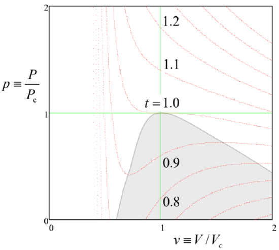
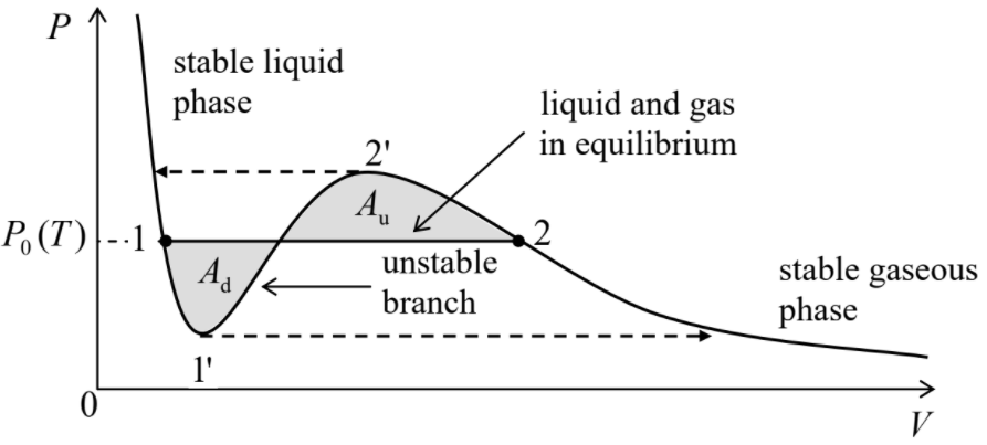
The most important property of these plots is that the isotherms have qualitatively different shapes in two temperature regions. At t>1, i.e. T>Tc, pressure increases monotonically at gas compression (qualitatively, as in an ideal classical gas, with P=NT/V, to which the van der Waals system tends at T>>Tc), i.e. with (∂P/∂V)T<0 at all points of the isotherm.5 However, below the critical temperature Tc, any isotherm features a segment with (∂P/∂V)T>0. It is easy to understand that, as least in a constant-pressure experiment (see, for example, Figure 1.4.1),6 these segments describe a mechanically unstable equilibrium. Indeed, if due to a random fluctuation, the volume deviated upward from the equilibrium value, the pressure would also increase, forcing the environment (say, the heavy piston in Figure 1.4.1) to allow further expansion of the system, leading to even higher pressure, etc. A similar deviation of volume downward would lead to a similar avalanche-like decrease of the volume. Such avalanche instability would develop further and further until the system has reached one of the stable branches with a negative slope (∂P/∂V)T. In the range where the single-phase equilibrium state is unstable, the system as a whole may be stable only if it consists of the two phases (one with a smaller, and another with a higher density n=N/V) that are described by the two stable branches – see Figure 4.1.2.
In order to understand the basic properties of this two-phase system, let us recall the general conditions of the thermodynamic equilibrium of two systems, which have been discussed in Chapter 1:
Phase equilibrium conditions:
T1=T2 (thermal equilibrium),
Phase equilibrium conditions:
μ1=μ2 (“chemical” equilibrium),
the latter condition meaning that the average energy of a single (“probe”) particle in both systems has to be the same. To those, we should add the evident condition of mechanical equilibrium,
Phase equilibrium conditions:
P1=P2 (mechanical equilibrium),
which immediately follows from the balance of normal forces exerted on an inter-phase boundary.
If we discuss isotherms, Equation (???) is fulfilled automatically, while Equation (???) means that the effective isotherm P(V) describing a two-phase system should be a horizontal line – see Figure 4.1.2:
P=P0(T).
Along this line,7 internal properties of each phase do not change; only the particle distribution is: it evolves gradually from all particles being in the liquid phase at point 1 to all particles being in the gas phase at point 2.8 In particular, according to Equation (???), the chemical potentials μ of the phases should be equal at each point of the horizontal line (???). This fact enables us to find the line's position: it has to connect points 1 and 2 in that the chemical potentials of the two phases are equal to each other. Let us recast this condition as
∫21dμ=0, i.e. ∫21dG=0,
where the integral may be taken along the single-phase isotherm. (For this mathematical calculation, the mechanical instability of states on some part of this curve is not important.) By its construction, along that curve, N= const and T= const, so that according to Equation (1.5.4), dG=–SdT+VdP+μdN, for a slow (reversible) change, dG=VdP. Hence Equation (???) yields
∫21VdP=0.
This equality means that in Figure 4.1.2, the shaded areas Ad and Au should be equal.9
As the same Figure 4.1.2 figure shows, the Maxwell rule may be rewritten in a different form,
Maxwell equal-area rule:
∫21[P−P0(T)]dV=0.
which is more convenient for analytical calculations than Equation (???) if the equation of state may be explicitly solved for P – as it is in the van der Waals model (???). Such calculation (left for the reader's exercise) shows that for that model, the temperature dependence of the saturated vapor pressure at low T is exponential,10
P0(T)∝Pcexp{−ΔT}, with Δ=ab≡278Tc, for T<<Tc,
corresponding very well to the physical picture of particle's thermal activation from a potential well of depth Δ.
The signature parameter of a first-order phase transition, the latent heat of evaporation
Latent heat: definition
Λ≡∫21dQ,
may also be found by a similar integration along the single-phase isotherm. Indeed, using Equation (1.3.6), dQ=TdS, we get
Λ=∫21TdS=T(S2−S1).
Let us express the right-hand side of Equation (???) via the equation of state. For that, let us take the full derivative of both sides of Equation (???) over temperature, considering the value of G=Nμ for each phase as a function of P and T, and taking into account that according to Equation (???), P1=P2=P0(T):
(∂G1∂T)P+(∂G1∂P)TdP0dT=(∂G2∂T)P+(∂G2∂P)TdP0dT.
According to the first of Eqs. (1.4.16), the partial derivative (∂G/∂T)P is just minus the entropy, while according to the second of those equalities, (∂G/∂P)T is the volume. Thus Equation (???) becomes
−S1+V1dP0dT=−S2+V2dP0dT.
Solving this equation for (S2–S1), and plugging the result into Equation (???), we get the following Clapeyron-Clausius formula:
Clapeyron-Clausius formula:
Λ=T(V2−V1)dP0dT.
For the van der Waals model, this formula may be readily used for the analytical calculation of Λ in two limits: T<<Tc and (Tc–T)<<Tc – the exercises left for the reader. In the latter limit, Λ∝(Tc–T)1/2, naturally vanishing at the critical temperature.
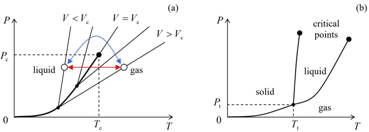
Finally, some important properties of the van der Waals' model may be revealed more easily by looking at the set of its isochores P=P(T) for V= const, rather than at the isotherms. Indeed, as Equation (???) shows, all single-phase isochores are straight lines. However, if we interrupt these lines at the points when the single phase becomes metastable, and complement them with the (very nonlinear!) dependence P0(T), we get the pattern (called the phase diagram) shown schematically in Figure 4.1.3a.
Thus, in the van der Waals model, two phases may coexist, though only at certain conditions – in particular, T<Tc. Now a natural, more general question is whether the coexistence of more than two phases of the same substance is possible. For example, can the water ice, the liquid water, and the water vapor (steam) all be in thermodynamic equilibrium? The answer is essentially given by Equation (???). From thermodynamics, we know that for a uniform system (i.e. a single phase), pressure and temperature completely define the chemical potential μ(P,T). Hence, dealing with two phases, we had to satisfy just one chemical equilibrium condition (???) for two common arguments P and T. Evidently, this leaves us with one extra degree of freedom, so that the two-phase equilibrium is possible within a certain range of P at fixed T (or vice versa) – see again the horizontal line in Figure 4.1.2 and the bold line in Figure 4.1.3a. Now, if we want three phases to be in equilibrium, we need to satisfy two equations for these variables:
μ1(P,T)=μ2(P,T)=μ3(P,T).
Typically, the functions μ(P,T) are monotonic, so that the two equations (???) have just one solution, the so-called triple point {Pt,Tt}. Of course, the triple point {Pt,Tt} of equilibrium between three phases should not be confused with the critical points {Pc,Tc} of transitions between each of two-phase pairs. Figure 4.1.3b shows, very schematically, their relation for a typical three-phase system solid-liquid-gas. For example, water, ice, and water vapor are at equilibrium at a triple point corresponding to Pt≈0.612 kPa13 and Tt=273.16 K. The practical importance of this particular temperature point is that by an international agreement it has been accepted for the definition of not only the Kelvin temperature scale, but also of the Celsius scale's reference, as 0.01∘C, so that the absolute temperature zero corresponds to exactly –273.15∘C.14 More generally, triple points of purified simple substances (such as H2, N2, O2, Ar, Hg, and H2O) are broadly used for thermometer calibration, defining the so-called international temperature scales including the currently accepted scale ITS-90.
This analysis may be readily generalized to multi-component systems consisting of particles of several (say, L) sorts.15 If such a mixed system is in a single phase, i.e. is macroscopically uniform, its chemical potential may be defined by a natural generalization of Equation (1.5.4):
dG=−SdT+VdP+L∑l=1μ(l)dN(l).
The last term reflects the fact that usually, each single phase is not a pure chemical substance, but has certain concentrations of all other components, so that μ(l) may depend not only on P and T but also on the concentrations c(l)≡N(l)/N of particles of each sort. If the total number N of particles is fixed, the number of independent concentrations is (L–1). For the chemical equilibrium of R phases, all R values of μ(l)r(r=1,2,...,R) have to be equal for particles of each sort: μ(l)1=μ(l)2=...=μ(l)R, with each μ(l)r depending on (L–1) concentrations c(l)r, and also on P and T. This requirement gives L(R–1) equations for (L–1)R concentrations c(l)r, plus two common arguments P and T, i.e. for [(L–1)R+2] independent variables. This means that the number of phases has to satisfy the limitation
Gibbs phase rule:
L(R−1)≤(L−1)R+2, i.e. R≤L+2,
where the equality sign may be reached in just one point in the whole parameter space. This is the Gibbs phase rule. As a sanity check, for a single-component system, L=1, the rule yields R≤3 – exactly the result we have already discussed.