
5.2: Energy and the number of particles


- Last updated
- Sep 20, 2022
- Save as PDF

( \newcommand{\kernel}{\mathrm{null}\,}\)
First of all, note that fluctuations of macroscopic variables depend on particular conditions.2 For example, in a mechanically- and thermally-insulated system with a fixed number of particles, i.e. a member of a microcanonical ensemble, the internal energy does not fluctuate: δE=0. However, if such a system is in thermal contact with the environment, i.e. is a member of a canonical ensemble (Figure 2.4.1), the situation is different. Indeed, for such a system we may apply the general Equation (2.1.7), with Wm given by the Gibbs distribution (2.4.7)-(2.4.8), not only to E but also to E2. As we already know from Sec. 2.4, the first average,
⟨E⟩=∑mWmEm,Wm=1Zexp{−EmT},Z=∑mexp{−EmT},
yields Equation (2.4.10), which may be rewritten in the form
⟨E⟩=1Z∂Z∂(−β), where β≡1T,
more convenient for our current purposes. Let us carry out a similar calculation for E2:
⟨E2⟩=∑mWmE2m=1Z∑mE2mexp{−βEm}.
It is straightforward to verify, by double differentiation, that the last expression may be rewritten in a form similar to Equation (???):
⟨E2⟩=1Z∂2∂(−β)2∑mexp{−βEm}≡1Z∂2Z∂(−β)2.
Now it is easy to use Eqs. (5.1.4−5.1.5) to calculate the variance of energy fluctuations:
⟨˜E2⟩=⟨E2⟩−⟨E⟩2=1Z∂2Z∂(−β)2−(1Z∂Z∂(−β))2≡∂∂(−β)(1Z∂Z∂(−β))=∂⟨E⟩∂(−β).
Since Eqs. (???)-(???) are valid only if the system's volume V is fixed (because its change may affect the energy spectrum Em), it is customary to rewrite this important result as follows:
Fluctuations of E:
⟨˜E2⟩=∂⟨E⟩∂(−1/T)=T2(∂⟨E⟩∂T)V≡CVT2.
This is a remarkably simple, fundamental result. As a sanity check, for a system of N similar, independent particles, ⟨E⟩ and hence CV are proportional to N, so that δE∝N1/2 and δE/⟨E⟩∝N–1/2, in agreement with Equation (5.1.13). Let me emphasize that the classically-looking Equation (???) is based on the general Gibbs distribution, and hence is valid for any system (either classical or quantum) in thermal equilibrium.
Some corollaries of this result will be discussed in the next section, and now let us carry out a very similar calculation for a system whose number N of particles in a system is not fixed, because they may go to, and come from its environment at will. If the chemical potential μ of the environment and its temperature T are fixed, i.e. we are dealing with the grand canonical ensemble (Figure 2.7.1), we may use the grand canonical distribution (2.7.5)-(2.7.6):
Wm,N=1ZGexp{μN−Em,NT},ZG=∑N,mexp{μN−Em,NT}.
Acting exactly as we did above for the internal energy, we get
⟨N⟩=1ZG∑m,NNexp{μN−Em,NT}=TZG∂ZG∂μ,
⟨N2⟩=1ZG∑m,NN2exp{μN−Em,NT}=T2ZG∂2ZG∂μ2,
so that the particle number's variance is
Fluctuations of N:
⟨˜N2⟩=⟨N2⟩−⟨N⟩2=T2ZG∂ZG∂μ−T2Z2G(∂ZG∂μ)2=T∂∂μ(TZG∂ZG∂μ)=T∂⟨N⟩∂μ,
in full analogy with Equation (???).
In particular, for an ideal classical gas, we may combine the last result with Equation (3.2.2). (As was already emphasized in Sec. 3.2, though that result has been obtained for the canonical ensemble, in which the number of particles N is fixed, at N>>1 the fluctuations of N in the grand canonical ensemble should be relatively small, so that the same relation should be valid for the average ⟨N⟩ in that ensemble.) Easily solving Equation (3.2.2) for ⟨N⟩, we get
⟨N⟩=const×exp{μT},
where “const” means a factor constant at the partial differentiation of ⟨N⟩ over μ, required by Equation (???). Performing the differentiation and then using Equation (???) again,
∂⟨N⟩∂μ=const×1Texp{μT}=⟨N⟩T,
we get from Equation (???) a very simple result:
Fluctuations of N: classical gas
⟨˜N2⟩=⟨N⟩, i.e. δN=⟨N⟩1/2.
This relation is so important that I will also show how it may be derived differently. As a by-product of this new derivation, we will prove that this result is valid for systems with an arbitrary (say, small) N, and also get more detailed information about the statistics of fluctuations of that number. Let us consider an ideal classical gas of N0 particles in a volume V0, and calculate the probability WN to have exactly N≤N0 of these particles in its part of volume V≤V0 – see Figure 5.2.1.
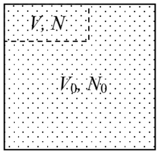
For one particle such probability is W=V/V0=⟨N⟩/N0≤1, while the probability to have that particle in the remaining part of the volume is W′=1–W=1–⟨N⟩/N0. If all particles were distinguishable, the probability of having N≤N0 specific particles in volume V and (N–N0) specific particles in volume (V–V0), would be WNW′(N0−N). However, if we do not want to distinguish the particles, we should multiply this probability by the number of possible particle combinations keeping the numbers N and N0 constant, i.e. by the binomial coefficient N0!/N!(N0–N)!.3 As the result, the required probability is
Binomial distribution:
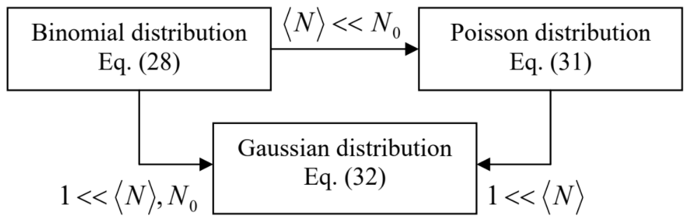
WN=WNW′(N0−N)N0!N!(N0−N)!=(⟨N⟩N0)N(1−⟨N⟩N0)N0−NN0!N!(N0−N)!.
This is the so-called binomial probability distribution, valid for any ⟨N⟩ and N0.4
Still keeping ⟨N⟩ arbitrary, we can simplify the binomial distribution by assuming that the whole volume V0, and hence N0, are very large:
N0>>N,
where N means all values of interest, including ⟨N⟩. Indeed, in this limit we can neglect N in comparison with N0 in the second exponent of Equation (???), and also approximate the fraction N0!/(N0–N)!, i.e. the product of N terms, (N0–N+1)(N0–N+2)...(N0–1)N0, by just NN0. As a result, we get
WN≈(⟨N⟩N0)N(1−⟨N⟩N0)N0NN0N!≡⟨N⟩NN!(1−⟨N⟩N0)N0=⟨N⟩NN![(1−W)1W]⟨N⟩,
where, as before, W=⟨N⟩/N0. In the limit (???), W→0, so that the factor inside the square brackets tends to 1/e, the reciprocal of the natural logarithm base.5 Thus, we get an expression independent of N0:
Poisson distribution:
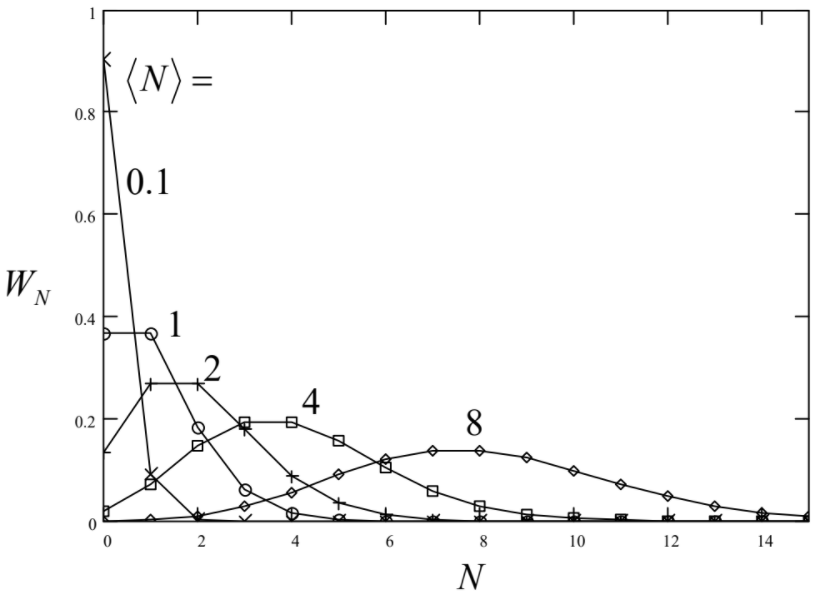
WN=⟨N⟩NN!e−⟨N⟩.
This is the much-celebrated Poisson distribution6 which describes a very broad family of random phenomena. Figure 5.2.2 shows this distribution for several values of ⟨N⟩ – which, in contrast to N, are not necessarily integer.
Gaussian distribution:
WN=1(2π)1/2δNexp{−(N−⟨N⟩)22(δN)2}.
(Note that the Gaussian distribution is also valid if both N and N0 are large, regardless of the relation between them – see Figure 5.2.3.)
A major property of the Poisson (and hence of the Gaussian) distribution is that it has the same variance as given by Equation (???):
⟨˜N2⟩≡⟨(N−⟨N⟩)2⟩=⟨N⟩.
(This is not true for the general binomial distribution.) For our current purposes, this means that for the ideal classical gas, Equation (???) is valid for any number of particles.