6.6: Exercise problems

Last updated
Save as PDF

Page ID: 34735

$ \newcommand{\vecs}[1]{\overset { \scriptstyle \rightharpoonup} {\mathbf{#1}} } $ $ \newcommand{\vecd}[1]{\overset{-\!-\!\rightharpoonup}{\vphantom{a}\smash {#1}}} $$\newcommand{\id}{\mathrm{id}}$ $ \newcommand{\Span}{\mathrm{span}}$ $ \newcommand{\kernel}{\mathrm{null}\,}$ $ \newcommand{\range}{\mathrm{range}\,}$ $ \newcommand{\RealPart}{\mathrm{Re}}$ $ \newcommand{\ImaginaryPart}{\mathrm{Im}}$ $ \newcommand{\Argument}{\mathrm{Arg}}$ $ \newcommand{\norm}[1]{\| #1 \|}$ $ \newcommand{\inner}[2]{\langle #1, #2 \rangle}$ $ \newcommand{\Span}{\mathrm{span}}$ $\newcommand{\id}{\mathrm{id}}$ $ \newcommand{\Span}{\mathrm{span}}$ $ \newcommand{\kernel}{\mathrm{null}\,}$ $ \newcommand{\range}{\mathrm{range}\,}$ $ \newcommand{\RealPart}{\mathrm{Re}}$ $ \newcommand{\ImaginaryPart}{\mathrm{Im}}$ $ \newcommand{\Argument}{\mathrm{Arg}}$ $ \newcommand{\norm}[1]{\| #1 \|}$ $ \newcommand{\inner}[2]{\langle #1, #2 \rangle}$ $ \newcommand{\Span}{\mathrm{span}}$$\newcommand{\AA}{\unicode[.8,0]{x212B}}$

Exercise $\PageIndex{1}$

Use the Boltzmann equation in the relaxation-time approximation to derive the Drude formula for the complex ac conductivity $\sigma (\omega )$, and give a physical interpretation of the result's trend at high frequencies.

Exercise $\PageIndex{2}$

Apply the variable separation method⁷⁶ to Equation ($6.3.15$) to calculate the time evolution of the particle density distribution in an unlimited uniform medium, in the absence of external forces, provided that at $t = 0$ the particles are released from their uniform distribution in a plane layer of thickness $2a$:

\[n = \begin{cases} n_0, & \text{ for } - a \leq x \leq + a, \\ 0, & \text{ otherwise.} \end{cases} \nonumber\]

Exercise $\PageIndex{3}$

Solve the previous problem using an appropriate Green's function for the 1D version of the diffusion equation, and discuss the relative convenience of the results.

Exercise $\PageIndex{4}^*$

Calculate the electric conductance of a narrow, uniform conducting link between two bulk conductors, in the low-voltage and low-temperature limit, neglecting the electron interaction and scattering inside the link.

Exercise $\PageIndex{5}$

Calculate the effective capacitance (per unit area) of a broad plane sheet of a degenerate 2D electron gas, separated by distance $d$ from a metallic ground plane.

Exercise $\PageIndex{6}$

Give a quantitative description of the dopant atom ionization, which would be consistent with the conduction and valence band occupation statistics, using the same simple model of an $n$-doped semiconductor as in Sec. 4 (see Figure $6.4.2a$), and taking into account that the ground state of the dopant atom is typically doubly degenerate, due to two possible spin orientations of the bound electron. Use the results to verify Equation ($6.4.13$), within the displayed limits of its validity.

Exercise $\PageIndex{7}$

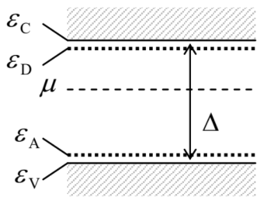
Generalize the solution of the previous problem to the case when the $n$-doping of a semiconductor by $n_D$ donor atoms per unit volume is complemented with its simultaneous $p$-doping by $n_A$ acceptor atoms per unit volume, whose energy $\varepsilon_A – \varepsilon_V$ of activation, i.e. of accepting an additional electron and hence becoming a negative ion, is much lower than the bandgap $\Delta$ – see the figure on the right.

Exercise $\PageIndex{8}$

A nearly-ideal classical gas of $N$ particles with mass $m$, was in thermal equilibrium at temperature $T$, in a closed container of volume $V$. At some moment, an orifice of a very small area $A$ is open in one of the container's walls, allowing the particles to escape into the surrounding vacuum.⁷⁷ In the limit of very low density $n \equiv N/V$, use simple kinetic arguments to calculate the r.m.s. velocity of the escaped particles during the time period when the total number of such particles is still much smaller than $N$. Formulate the limits of validity of your results in terms of $V$, $A$, and the mean free path $l$.

Hint: Here and below, the term “nearly-ideal” means that $l$ is so large that particle collisions do not affect the basic statistical properties of the gas.

Exercise $\PageIndex{9}$

For the system analyzed in the previous problem, calculate the rate of particle flow through the orifice – the so-called effusion rate. Discuss the limits of validity of your result.

Exercise $\PageIndex{10}$

Use simple kinetic arguments to estimate:

the diffusion coefficient $D$,
the thermal conductivity $\kappa $, and
the shear viscosity $\eta $,

of a nearly-ideal classical gas with mean free path $l$. Compare the result for $D$ with that calculated in Sec. 3 from the Boltzmann-RTA equation.

\[\frac{d\mathscr{F}_{j'}}{dA_j} = \eta \frac{\partial v_{j'}}{\partial r_j}, \nonumber\]

where $d\mathscr{F}_{j'}$ is the $j'^{ th}$ Cartesian component of the tangential force between two parts of a fluid, separated by an imaginary interface normal to some direction $\mathbf{n}_j$ (with $j \neq j'$, and hence $\mathbf{n}_j \perp \mathbf{n}_{j'}$), exerted over an elementary area $dA_j$ of this surface, and $\mathbf{v}(\mathbf{r})$ is the velocity of the fluid at the interface.

Exercise $\PageIndex{11}$

Use simple kinetic arguments to relate the mean free path $l$ in a nearly-ideal classical gas, with the full cross-section $\sigma$ of mutual scattering of its particles.⁷⁹ Use the result to evaluate the thermal conductivity and the viscosity coefficient estimates made in the previous problem, for the molecular nitrogen, with the molecular mass $m \approx 4.7 \times 10^{-26}$ kg and the effective (“van der Waals”) diameter $d_{ef} \approx 4.5 \times 10^{-10}$ m, at ambient conditions, and compare them with experimental results.

Exercise $\PageIndex{12}$

Use the Boltzmann-RTA equation to calculate the thermal conductivity of a nearly-ideal classical gas, measured in conditions when the applied thermal gradient does not create a net particle flow. Compare the result with that following from the simple kinetic arguments (Problem 6.10), and discuss their relationship.

Exercise $\PageIndex{13}$

Use the heat conduction equation ($6.5.26$) to calculate the time evolution of temperature in the center of a uniform solid sphere of radius $R$, initially heated to a uniformly distributed temperature $T_{ini}$, and at $t = 0$ placed into a heat bath that keeps its surface at temperature $T_0$.

Exercise $\PageIndex{14}$

Suggest a reasonable definition of the entropy production rate (per unit volume), and calculate this rate for stationary thermal conduction, assuming that it obeys the Fourier law, in a material with negligible thermal expansion. Give a physical interpretation of the result. Does the stationary temperature distribution in a sample correspond to the minimum of the total entropy production in it?

Exercise $\PageIndex{15}$⁸⁰

Use the Boltzmann-RTA equation to calculate the shear viscosity of a nearly-ideal gas. Spell out the result in the classical limit, and compare it with the estimate made in the solution of Problem 10.

This topic was briefly addressed in EM Chapter 4, carefully avoiding the aspects related to the thermal effects.
See, e.g., CM Sec. 10.1.
Actually, this is just one of several theorems bearing the name of Joseph Liouville (1809-1882).
See, e.g., MA Equation (4.2).
See, e.g., CM Sec. 9.3.
Indeed, the quantum state coherence is described by off-diagonal elements of the density matrix, while the classical probability $w$ represents only the diagonal elements of that matrix. However, at least for the ensembles close to thermal equilibrium, this is a reasonable approximation – see the discussion in Sec. 2.1.
One may wonder whether this approximation may work for Fermi particles, such as electrons, for whom the Pauli principle forbids scattering into the already occupied state, so that for the scattering $\mathbf{p} \rightarrow \mathbf{p}'$, the term $w(\mathbf{r}, \mathbf{p}, t)$ in Equation ($6.1.12$) has to be multiplied by the probability $[1 – w(\mathbf{r}, \mathbf{p}', t)]$ that the final state is available. This is a valid argument, but one should notice that if this modification has been done with both terms of Equation ($6.1.12$), it becomes \[ \left| \frac{\partial w}{\partial t} \right|_{scattering} = \int d^3 p' \Gamma_{\mathbf{p} \rightarrow \mathbf{p}'} \{ w (\mathbf{r},\mathbf{p}',t) [ \mathbf{1} - w(\mathbf{r},\mathbf{p},t)]-w(\mathbf{r},\mathbf{p},t)[\mathbf{1}-w(\mathbf{r},\mathbf{p}',t)]\}.\nonumber\] Opening both square brackets, we see that the probability density products cancel, bringing us back to Equation ($6.1.12$).
This was the approximation used by L. Boltzmann to prove the famous $H$-theorem, stating that entropy of the gas described by Equation ($6.1.13$) may only grow (or stay constant) in time, $dS/dt \geq 0$. Since the model is very approximate, that result does not seem too fundamental nowadays, despite all its historic significance.
Sometimes this approximation is called the “BGK model”, after P. Bhatnager, E. Gross, and M. Krook who suggested it in 1954. (The same year, a similar model was considered by P. Welander.)
See, e.g., CM Sec. 3.7.
Since the scale of the fastest change of $w_0$ in the momentum space is of the order of $\partial w_0/\partial p = (\partial w_0/\partial \varepsilon )(d\varepsilon /dp) \sim (1/T)v$, where $v$ is the scale of particle's speed, the necessary condition of the linear approximation ($6.2.4$) is $e\mathscr{E}\tau << T/v$, i.e. if $e\mathscr{E}l << T$, where $l \equiv v\tau$ has the meaning of the effective mean-free path. Since the left-hand side of the last inequality is just the average energy given to the particle by the electric field between two scattering events, the condition may be interpreted as the smallness of the gas' “overheating” by the applied field. However, another condition is also necessary – see the last paragraph of this section.
See, e.g., QM Sec. 2.1.
It was obtained by Arnold Sommerfeld in 1927.
See, e.g., QM Secs. 2.7, 2.8, and 3.4. (In this case, $\mathbf{p}$ should be understood as the quasimomentum rather than the genuine momentum.)
As Equation ($6.2.9$) shows, if the dispersion law $\varepsilon (\mathbf{p})$ is anisotropic, the current density direction may be different from that of the electric field. In this case, conductivity should be described by a tensor $\sigma_{jj'}$, rather than a scalar. However, in most important conducting materials, the anisotropy is rather small – see, e.g., EM Table 4.1.
This is why to determine the dominating type of charge carriers in semiconductors (electrons or holes, see Sec. 4 below), the Hall effect, which lacks such ambivalence (see, e.g., QM 3.2), is frequently used.
It was derived in 1900 by Paul Drude. Note that Drude also used the same arguments to derive a very simple (and very reasonable) approximation for the complex electric conductivity in the ac field of frequency $\omega : \sigma (\omega ) = \sigma (0)/(1 – i\omega \tau )$, with $\sigma (0)$ given by Equation ($6.2.14$); sometimes the name “Drude formula” is used for this expression rather than for Equation ($6.2.14$). Let me leave its derivation, from the Boltzmann-RTA equation, for the reader's exercise.
See also EM Sec. 4.2.
So here, as it frequently happens in physics, formulas (or graphical sketches, such as Figure $6.2.1b$) give a more clear and unambiguous description of reality than words – the privilege lacked by many “scientific” disciplines, rich with unending, shallow verbal debates. Note also that, as frequently happens in physics, the dual interpretation of $\sigma$ is expressed by two different but equal integrals ($6.2.12$) and ($6.2.13$), related by the integration-by-parts rule.
This formula is probably self-evident, but if you need you may revisit EM Sec. 4.4.
Since we will not encounter $\nabla_p$ in the balance of this chapter, from this point on, the subscript $r$ of the operator $\nabla_r$ is dropped for the notation brevity.
Since we consider $w_0$ as a function of two independent arguments $\mathbf{r}$ and $\mathbf{p}$, taking its gradient, i.e. the differentiation of this function over $\mathbf{r}$, does not involve its differentiation over the kinetic energy $\varepsilon$ – which is a function of $\mathbf{p}$ only.
Note that Equation ($6.3.7$) does not include the phenomenological parameter $\tau$ of the relaxation-time approximation, signaling that it is much more general than the RTA. Indeed, this equality is based entirely on the relation between the second and third terms on the left-hand side of the general Boltzmann equation ($6.1.10$), rather than on any details of the scattering integral on its right-hand side.
Sometimes it is also called the “electron affinity”, though this term is mostly used for atoms and molecules.
In semiconductor physics and engineering, the situation shown in Figure $6.3.1b$ is called the flat-band condition, because any electric field applied normally to a surface of a semiconductor leads to the so-called energy band bending – see the next section.
As measured from a common reference value, for example from the vacuum level – rather than from the bottom of an individual potential well as in Figure $6.3.1a$.
In physics literature, it is usually called the contact potential difference, while in electrochemistry (for which it is one of the key notions), the term Volta potential is more common.
The devices for such measurement may be based on the interaction between the measured current and a permanent magnet, as pioneered by A.-M. Ampère in the 1820s – see, e.g., EM Chapter 5. Such devices are sometimes called galvanometers, honoring another pioneer of electricity, Luigi Galvani.
If this relation is not evident, please revisit EM Sec. 4.1.
Sometimes this term is associated with Equation ($6.3.19$). One may also run into the term “convection-diffusion equation” for Equation ($6.3.15$) with the replacement ($6.3.16$).
And hence, at negligible $\nabla U$, identical to the diffusion equation ($5.6.11$).
See, e.g., QM Sec. 2.7 and 3.4, but the thorough knowledge of this material is not necessary for following discussions of this section. If the reader is not familiar with the notion of quasimomentum (alternatively called the “crystal momentum”), its following semi-quantitative interpretation may be useful: $\mathbf{q}$ is the result of quantum averaging of the genuine electron momentum $\mathbf{p}$ over the crystal lattice period. In contrast to $\mathbf{p}$, which is not conserved because of the electron's interaction with the atomic lattice, $\mathbf{q}$ is an integral of motion – in the absence of other forces.
In insulators, the bandgap $\Delta$ is so large (e.g., $\sim 9$ eV in $\ce{SiO2}$) that the conduction band remains unpopulated in all practical situations, so that the following discussion is only relevant for semiconductors, with their moderate bandgaps – such as 1.14 eV in the most important case of silicon at room temperature.
It is easy (and hence is left for the reader's exercise) to verify that all equilibrium properties of charge carriers remain the same (with some effective values of $m_C$ and $m_V$) if $\varepsilon_c(\mathbf{q})$ and $\varepsilon_v(\mathbf{q})$ are arbitrary quadratic forms of the Cartesian components of the quasimomentum. A mutual displacement of the branches $ \varepsilon_c(\mathbf{q})$ and $\varepsilon_v(\mathbf{q}$) in the quasimomentum space is also unimportant for statistical and most transport properties of the semiconductors, though it is very important for their optical properties – which I will not have time to discuss in any detail.
The collective name for them in semiconductor physics is charge carriers – or just “carriers”.
Note that in the case of simple electron spin degeneracy ($g_V = g_C = 2$), the first logarithm vanishes altogether. However, in many semiconductors, the degeneracy is factored by the number of similar energy bands (e.g., six similar conduction bands in silicon), and the factor $\ln (g_V/g_C)$ may slightly affect quantitative results.
Note that in comparison with Figure $6.4.1$, here the (for most purposes, redundant) information on the $q$-dependence of the energies is collapsed, leaving the horizontal axis of such a band-edge diagram free for showing their possible spatial dependences – see Figs. $6.4.3$, $6.4.5$, and $6.4.6$ below.
Very similar relations may be met in the theory of chemical reactions (where it is called the law of mass action), and other disciplines – including such exotic examples as the theoretical ecology.
Let me leave it for the reader's exercise to prove that this assumption is always valid unless the doping density $n_D$ becomes comparable to $n_C$, and as a result, the Fermi energy $\mu$ moves into a $\sim T$-wide vicinity of $\varepsilon_D$.
For the typical donors (P) and acceptors (B) in silicon, both ionization energies, ($\varepsilon_C – \varepsilon_D)$ and $(\varepsilon_A – \varepsilon_V$), are close to 45 meV, i.e. are indeed much smaller than $\Delta \approx 1.14$ eV.
A simplified version of this analysis was discussed in EM Sec. 2.1.
See, e.g., EM Sec. 3.4.
I am sorry for using, for the SI electric constant $\varepsilon_0$, the same Greek letter as for single-particle energies, but both notations are traditional, and the difference between these uses will be clear from the context.
It is common (though not necessary) to select the energy reference so that deep inside the semiconductor, $\phi = 0$; in what follows I will use this convention.
Here $\mathscr{E}$ is the field just inside the semiconductor. The free-space field necessary to create it is $\kappa$ times larger – see, e.g., the same EM Sec. 3.4, in particular Equation ($3.3.5$).
In semiconductor physics literature, the value of $\mu '$ is usually called the Fermi level, even in the absence of the degenerate Fermi sea typical for metals – cf. Sec. 3.3. In this section, I will follow this common terminology.
Even some amorphous thin-film insulators, such as properly grown silicon and aluminum oxides, can withstand fields up to $\sim 10$ MV/cm.
As a reminder, the derivation of this formula was the task of Problem 3.14.
The classical monograph in this field is S. Sze, Physics of Semiconductor Devices, $2^{nd}$ ed., Wiley 1981. (The $3^{rd}$ edition, circa 2006, co-authored with K. Ng, is more tilted toward technical details.) I can also recommend a detailed textbook by R. Pierret, Semiconductor Device Fundamentals, $2^{nd}$ ed., Addison Wesley, 1996.
Frequently, Equation ($6.4.30$) is also rewritten in the form $e\Delta \varphi = T \ln (n_Dn_A/n_i^2)$. In the view of the second of Eqs. ($6.4.8$), this equality is formally correct but may be misleading because the intrinsic carrier density $n_i$ is an exponential function of temperature and is physically irrelevant for this particular problem.
Note that such $w$ is again much larger than $\lambda_D$ – the fact that justifies the first two boundary conditions ($6.4.32$).
Another important limit is quantum-mechanical tunneling through the gate insulator, whose thickness has to be scaled down in parallel with lateral dimensions of a FET, including its channel length.
In the semiconductor physics lingo, the “carrier generation” event is the thermal excitation of an electron from the valence band to the conduction band, leaving a hole behind, while the reciprocal event of filling such a hole by a conduction-band electron is called the “carrier recombination”.
Note that if an external photon with energy $\hbar \omega > \Delta$ generates an electron-hole pair somewhere inside the depletion layer, this electric field immediately drives its electron component to the right, and the hole component to the left, thus generating a pulse of electric current through the junction. This is the physical basis of the whole vast technological field of photovoltaics, currently strongly driven by the demand for renewable electric power. Due to the progress of this technology, the cost of solar power systems has dropped from ~$300 per watt in the mid-1950s to the current ~$1 per watt, and its global generation has increased to almost 1015 watt-hours per year – though this is still below 2% of the whole generated electric power.
I will not try to reproduce this calculation (which may be found in any of the semiconductor physics books mentioned above), because getting all its scaling factors right requires using some model of the recombination process, and in this course, there is just no time for their quantitative discussion. However, see Equation ($6.4.42$) below.
In our model, the positive sign of $V \equiv \Delta \mu '/q \equiv –\Delta \mu '/e$ corresponds to the additional electric field, $–\nabla \mu '/q \equiv \nabla \mu '/e$, directed in the positive direction of the $x$-axis (in Figure $6.4.6$, from the left to the right), i.e. to the positive terminal of the voltage source connected to the p-doped semiconductor – which is the common convention.
This change, schematically shown in Figure $6.4.6b$, may be readily calculated by making the replacement ($6.4.37$) in the first of Eqs. ($6.4.34$).
This sign invariance may look strange, due to the opposite (positive) electric charge of the holes. However, this difference in the charge sign is compensated by the opposite direction of the hole diffusion – see Figure $6.4.5$. (Note also that the actual charge carriers in the valence band are still electrons, and the positive charge of holes is just a convenient representation of the specific dispersion law in this energy band, with a negative effective mass – see Figure $6.4.1$, the second line of Equation ($6.4.1$), and a more detailed discussion of this issue in QM Sec. 2.8.)
Some metal-semiconductor junctions, called Schottky diodes, have similar rectifying properties (and may be better fitted for high-power applications than silicon $p-n$ junctions), but their properties are more complex because of the rather involved chemistry and physics of interfaces between different materials.
See, e.g., the monograph by R. Stratonovich cited in Sec. 4.2.
Named after Thomas Johann Seebeck who experimentally discovered, in 1822, the effect described by the second term in Equation ($6.5.4$) – and hence by Equation ($6.5.10$).
Again, such independence hints that Equation ($6.5.8$) has a broader validity than in our simple model of an isotropic gas. This is indeed the case: this result turns out to be valid for any form of the Fermi surface, and for any dispersion law $\varepsilon (\mathbf{p})$. Note, however, that all calculations of this section are valid for the simplest RTA model in that $\tau$ is an energy-independent parameter; for real metals, a more accurate description of experimental results may be obtained by tweaking this model to take this dependence into account – see, e.g., Chapter 13 in the monograph by N. Ashcroft and N. D. Mermin, cited in Sec. 3.5.
Both these materials are alloys, i.e. solid solutions: chromel is 10% chromium in 90% nickel, while constantan is 45% nickel and 55% copper.
An alternative explanation of the factor $(\varepsilon – \mu )$ in Equation ($6.5.11$) is that according to Eqs. ($1.4.14$) and ($1.5.7$), for a uniform system of $N$ particles this factor is just $(E – G)/N \equiv (TS – PV)/N$. The full differential of the numerator is $TdS + SdT –PdV – VdP$, so that in the absence of the mechanical work $d\mathscr{W} = –PdV$, and changes of temperature and pressure, it is just $TdS \equiv dQ$ – see Equation ($1.3.6$).
Named after Jean Charles Athanase Peltier who experimentally discovered, in 1834, the effect expressed by the first term in Equation ($6.5.12$) – and hence by Equation ($6.5.19$).
See, for example, Sec. 15.7 in R. Pathria and P. Beale, Statistical Mechanics, $3^{rd}$ ed., Elsevier, 2011. Note, however, that the range of validity of the Onsager relations is still debated – see, e.g., K.-T. Chen and P. Lee, Phys. Rev. B 79, 18 (2009).
It was named after Gustav Wiedemann and Rudolph Franz who noticed the constancy of ratio $\kappa /\sigma$ for various materials, at the same temperature, as early as 1853. The direct proportionality of the ratio to the absolute temperature was noticed by Ludwig Lorenz in 1872. Due to his contribution, the Wiedemann-Franz law is frequently represented, in the SI temperature units, as $\kappa /\sigma = LT_K$, where the constant $L \equiv (\pi^2/3)k_B/e^2$, called the Lorenz number, is close to $2.45 \times 10^{-8}W\cdot \Omega \cdot K^{-2}$. Theoretically, Equation ($6.5.17$) was derived in 1928 by A. Sommerfeld.
Let me emphasize that here we are discussing the heat transferred through a conductor, not the Joule heat generated in it by the current. (The latter effect is quadratic, rather than linear, in current, and hence is much smaller at $I \rightarrow 0$.)
See, e.g., D. Rowe (ed.), Thermoelectrics Handbook: Macro to Nano, CRC Press, 2005.
It was suggested (in 1822) by the same universal scientific genius J.-B. J. Fourier who has not only developed such a key mathematical tool as the Fourier series but also discovered what is now called the greenhouse effect!
They are all similar to continuity equations for other quantities – e.g., the mass (see CM Sec. 8.3) and the quantum-mechanical probability (see QM Secs. 1.4 and 9.6).
According to Equation ($1.4.2$), in the case of negligible thermal expansion, it does not matter whether we speak about the internal energy $E$ or the enthalpy $H$.
If the dependence of $c_V$ on temperature may be ignored only within a limited temperature interval, Eqs. ($6.5.23$) and ($6.5.25$) may be still used within that interval, for temperature deviations from some reference value.
I hope the reader knows it by heart by now, but if not – see, e.g., MA Equation (12.2).
A much more detailed coverage of this important part of physics may be found, for example, in the textbook by L. Pitaevskii and E. Lifshitz, Physical Kinetics, Butterworth-Heinemann, 1981. A deeper discussion of the Boltzmann equation is given, e.g., in the monograph by S. Harris, An Introduction to the Theory of the Boltzmann Equation, Dover 2011. For a discussion of applied aspects of kinetics see, e.g., T. Bergman et al., Fundamentals of Heat and Mass Transfer, $7^{th}$ ed., Wiley, 2011.
A detailed introduction to this method (repeatedly used in this series) may be found, for example, in EM Sec. 2.5.
In chemistry-related fields, this process is frequently called effusion.
See, e.g., CM Equation (8.56). Please note the difference between the shear viscosity coefficient $\eta$ considered in this problem and the drag coefficient $\eta$ whose calculation was the task of Problem 3.2. Despite the similar (traditional) notation, and belonging to the same realm (kinematic friction), these coefficients have different definitions and even different dimensionalities.
I am sorry for using the same letter for the cross-section as for the electric Ohmic conductivity. (Both notations are very traditional.) Let me hope this would not lead to confusion, because the conductivity is not discussed in this problem.
This problem does not follow Problem 12 only for historic reasons.

Exercise \(\PageIndex{1}\)

Exercise \(\PageIndex{2}\)

Exercise \(\PageIndex{3}\)

Exercise \(\PageIndex{4}^*\)

Exercise \(\PageIndex{5}\)

Exercise \(\PageIndex{6}\)

Exercise \(\PageIndex{7}\)

Exercise \(\PageIndex{8}\)

Exercise \(\PageIndex{9}\)

Exercise \(\PageIndex{10}\)

Exercise \(\PageIndex{11}\)

Exercise \(\PageIndex{12}\)

Exercise \(\PageIndex{13}\)

Exercise \(\PageIndex{14}\)

Exercise \(\PageIndex{15}\)80

Exercise \(\PageIndex{15}\)⁸⁰