5.1: Space Translation Invariance

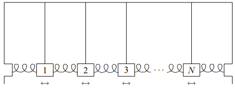
Figure \( 5.1\): A finite system of coupled pendulums.

The typical system of coupled oscillators that supports waves is one like the system of \(N\) identical coupled pendulums shown in Figure \( 5.1\). This system is a generalization of the system of two coupled pendulums that we studied in chapters 3 and 4. Suppose that each pendulum bob has mass \(m\), each pendulum has length \(\ell\), each spring has spring constant \(\kappa\) and the equilibrium separation between bobs is \(a\). Suppose further that there is no friction and that the pendulums are constrained to oscillate only in the direction in which the springs are stretched. We are interested in the free oscillation of this system, with no external force. Such an oscillation, when the motion is parallel to the direction in which the system is stretched in space is called a “longitudinal oscillation”. Call the longitudinal displacement of the \(j\)th bob from equilibrium (\psi_{j}\). We can organize the displacements into a vector, \(\Psi\) (for reasons that will become clear below, it would be confusing to use \(X\), so we choose a different letter, the Greek letter psi, which looks like \(\psi\) in lower case and \(\Psi\) when capitalized): \[\Psi=\left(\begin{array}{c}
\psi_{1} \\
\psi_{2} \\
\psi_{3} \\
\vdots \\
\psi_{N}
\end{array}\right) .\]

Then the equations of motion (for small longitudinal oscillations) are \[\frac{d^{2} \Psi}{d t^{2}}=-M^{-1} K \Psi\]

where \(M\) is the diagonal matrix with \(m\)’s along the diagonal, \[\left(\begin{array}{ccccc}
m & 0 & 0 & \cdots & 0 \\
0 & m & 0 & \cdots & 0 \\
0 & 0 & m & \cdots & 0 \\
\vdots & \vdots & \vdots & \ddots & \vdots \\
0 & 0 & 0 & \cdots & m
\end{array}\right) ,\]

and \(K\) has diagonal elements \((m g / \ell+2 \kappa)\), next-to-diagonal elements \(-\kappa\), and zeroes elsewhere, \[\left(\begin{array}{ccccc}
m g / \ell+2 \kappa & -\kappa & 0 & \cdots & 0 \\
-\kappa & m g / \ell+2 \kappa & -\kappa & \cdots & 0 \\
0 & -\kappa & m g / \ell+2 \kappa & \cdots & 0 \\
\vdots & \vdots & \vdots & \ddots & \vdots \\
0 & 0 & 0 & \cdots & m g / \ell+2 \kappa
\end{array}\right) .\]

The \(- \kappa\) in the next-to-diagonal elements has exactly the same origin as the \(- \kappa\) in the \(2 \times 2 \text { } K\) matrix in (3.78). It describes the coupling of two neighboring blocks by the spring. The \((m g / \ell+2 \kappa)\) on the diagonal is analogous to the \((m g / \ell+ \kappa)\) on the diagonal of (3.78). The difference in the factor of 2 in the coefficient of \(\kappa\) arises because there are two springs, one on each side, that contribute to the restoring force on each block in the system shown in Figure \( 5.1\), while there was only one in the system shown in Figure \( 3.1\). Thus \(M^{- 1}K\) has the form \[\left(\begin{array}{ccccc}
2 B & -C & 0 & \cdots & 0 \\
-C & 2 B & -C & \cdots & 0 \\
0 & -C & 2 B & \cdots & 0 \\
\vdots & \vdots & \vdots & \ddots & \vdots \\
0 & 0 & 0 & \cdots & 2 B
\end{array}\right)\]

where \[2 B=g / \ell+2 \kappa / m, \quad C=\kappa / m .\]

It is interesting to compare the matrix, (5.5), with the matrix, (4.43), from the previous chapter. In both cases, the diagonal elements are all equal, because of the symmetry. The same goes for the next-to-diagonal elements. However, in (5.5), all the rest of the elements are zero because the interactions are only between nearest neighbor blocks. We call such interactions “local.” In (4.43), on the other hand, each of the masses interacts with all the others. We will use the local nature of the interactions below.

We could try to find normal modes of this system directly by finding the eigenvectors of \(M^{- 1}K\), but there is a much easier and more generally useful technique. We can divide the physics of the system into two parts, the physics of the coupled pendulums, and the physics of the walls. To do this, we first consider an infinite system with no walls at all.

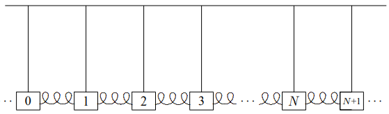
Figure \( 5.2\): A piece of an infinite system of coupled pendulums.

Notice that in Figure \( 5.2\), we have not changed the interior of the system shown in Figure \( 5.1\) at all. We have just replaced the walls by a continuation of the interior.

Now we can find all the modes of the infinite system of Figure \( 5.2\) very easily, making use of a symmetry argument. The infinite system of Figure \( 5.2\) looks the same if it is translated, moved to the left or the right by a multiple of the equilibrium separation, \(a\). It has the property of “space translation invariance.” Space translation invariance is the symmetry of the infinite system under translations by multiples of \(a\). In this example, because of the discrete blocks and finite length of the springs, the space translation invariance is “discrete.” Only translation by integral multiples of \(a\) give the same physics. Later, we will discuss continuous systems that have continuous space translation invariance. However, we will see that such systems can be analyzed using the same techniques that we introduce in this chapter.

We can use the symmetry of space translation invariance, just as we used the reflection and rotation symmetries discussed in the previous chapter, to find the normal modes of the infinite system. The discrete space translation invariance of the infinite system (the symmetry under translations by multiples of \(a\)) allows us to find the normal modes of the infinite system in a simple way.

Most of the modes that we find using the space translation invariance of the infinite system of Figure \( 5.2\) will have nothing to do with the finite system shown in Figure \( 5.1\). But if we can find linear combinations of the normal modes of the infinite system of Figure \( 5.2\) in which the 0th and \(N\) + 1st blocks stay fixed, then they must be solutions to the equations of motion of the system shown in Figure \( 5.1\). The reason is that the interactions between the blocks are “local” — they occur only between nearest neighbor blocks. Thus block 1 knows what block 0 is doing, but not what block −1 is doing. If block 0 is stationary it might as well be a wall because the blocks on the other side do not affect block 1 (or any of the blocks 1 to \(N\)) in any way. The local nature of the interaction allows us to put in the physics of the walls as a boundary condition after solving the infinite problem. This same trick will also enable us to solve many other problems.

Let us see how it works for the system shown in Figure \( 5.1\). First, we use the symmetry under translations to find the normal modes of the infinite system of Figure \( 5.2\). As in the previous two chapters, we describe the solutions in terms of a vector, \(A\). But now \(A\) has an infinite number of components, \(A_{j}\) where the integer \(j\) runs from \(- \infty\) to \(+ \infty\). It is a little inconvenient to write this infinite vector down, but we can represent a piece of it: \[A=\left(\begin{array}{c}
\vdots \\
A_{0} \\
A_{1} \\
A_{2} \\
A_{3} \\
\vdots \\
A_{N} \\
A_{N+1} \\
\vdots
\end{array}\right) .\]

Likewise, the \(M^{- 1}K\) matrix for the system is an infinite matrix, not easily written down, but any piece of it (along the diagonal) looks like the interior of (5.5): \[\left(\begin{array}{cccccc}
\ddots & \vdots & \vdots & \vdots & \vdots & \ddots \\
\cdots & 2 B & -C & 0 & 0 & \cdots \\
\cdots & -C & 2 B & -C & 0 & \cdots \\
\cdots & 0 & -C & 2 B & -C & \cdots \\
\cdots & 0 & 0 & -C & 2 B & \cdots \\
\ddots & \vdots & \vdots & \vdots & \vdots & \ddots
\end{array}\right) .\]

This system is “space translation invariant” because it looks the same if it is moved to the left a distance \(a\). This moves block \(j+1\) to where block \(j\) used to be, thus if there is a mode with components \(A_{j}\), there must be another mode with the same frequency, represented by a vector, \(A^{\prime} = SA|), with components \[A_{j}^{\prime}=A_{j+1} .\]

The symmetry matrix, \(S\), is an infinite matrix with 1s along the next-to-diagonal. These are analogous to the 1s along the next-to-diagonal in (4.40). Now, however, the transformation never closes on itself. There is no analog of the 1 in the lower left-hand corner of (4.40), because the infinite matrix has no corner. We want to find the eigenvalues and eigenvectors of the matrix \(S\), satisfying \[A^{\prime}=S A=\beta A\]

or equivalently (from (5.9)), the modes in which \(A_{j}\) and \(A_{j}^{\prime}\) are proportional: \[A_{j}^{\prime}=\beta A_{j}=A_{j+1}\]

where \(\beta\) is some nonzero constant.¹

Equation (5.11) can be solved as follows: Choose \(A_{0} = 1\). Then \(A_{1} = \beta\), \(A_{2} = \beta^{2}, etc., so that \(A_{j} = (\beta)^{j}\) for all nonnegative \(j\). We can also rewrite (5.11) as \(A_{j-1}=\beta^{-1} A_{j}\), so that \(A_{-1} = \beta_{-1\), \(A_{-2} = \beta_{-2}\), etc. Thus the solution is \[A_{j}=(\beta)^{j}\]

Now that we know the form of the normal modes, it is easy to get the corresponding frequencies by acting on (5.12) with the \(M^{-1}K\) matrix, (5.8). This gives \[\omega^{2} A_{j}^{\beta}=2 B A_{j}^{\beta}-C A_{j+1}^{\beta}-C A_{j-1}^{\beta} ,\]

or inserting (5.13), \[\omega^{2} \beta^{j}=2 B \beta^{j}-C \beta^{j+1}-C \beta^{j-1}=\left(2 B-C \beta-C \beta^{-1}\right) \beta^{j} .\]

This is true for all \(j\), which shows that (5.13) is indeed an eigenvector (we already knew this from the symmetry argument, (4.22), but it is nice to check when possible), and the eigenvalue is \[\omega^{2}=2 B-C \beta-C \beta^{-1} .\]

Notice that for almost every value of \(\omega^{2}\), there are two normal modes, because we can interchange \(\beta\) and \(\beta^{-1}\) without changing (5.16). The only exceptions are \[\omega^{2}=2 B \mp 2 C ,\]

corresponding to \(\beta=\pm 1\). The fact that there are at most two normal modes for each value of \(\omega^{2}\) will have a dramatic consequence. It means that we only have to deal with two normal modes at a time to implement the physics of the boundary. This is a special feature of the one-dimensional system that is not shared by two- and three-dimensional systems. As we will see, it makes the one-dimensional system very easy to handle.

Boundary Conditions

5-1
We have now solved the problem of the oscillation of the infinite system. Armed with this result, we can put back in the physics of the walls. Any \(\beta\) (except \(\beta=\pm 1\)) gives a pair of normal modes for the infinite system of Figure \( 5.2\). But only special values of \(\beta\) will work for the finite system shown in Figure \( 5.1\). To find the normal modes of the system shown in Figure \( 5.1\), we use (4.56), the fact that any linear combination of the two normal modes with the same angular frequency, \(\omega\), is also a normal mode. If we can find a linear combination that vanishes for \(j = 0\) and for \(j = N + 1\), it will be a normal mode of the system shown in Figure \( 5.1\). It is the vanishing of the normal mode at \(j = 0\) and \(j = N + 1\) that are the “boundary conditions” for this particular finite system.

Let us begin by trying to satisfy the boundary condition at \(j = 0\). For each possible value of \(\omega^{2}\), we have to worry about only two normal modes, the two solutions of (5.16) for \(\beta\). So long as \(\beta \neq \pm 1\), we can find a combination that vanishes at \(j = 0\); just subtract the two modes \(A^{\beta}\) and \(A^{\beta^{-1}}\) to get a vector \[A=A^{\beta}-A^{\beta^{-1}} ,\]

or in components \[A_{j} \propto A_{j}^{\beta}-A_{j}^{\beta^{-1}}=\beta^{j}-\beta^{-j} .\]

The first thing to notice about (5.19) is that \(A^{j}\) cannot vanish for any \(j \neq 0\) unless \(|\beta|=1\). Thus if we are to have any chance of satisfying the boundary condition at \(j = N + 1\), we must assume that \[\beta=e^{i \theta} .\]

Then from (5.19), \[A_{j} \propto \sin j \theta .\]

Now we can satisfy the boundary condition at \(j = N + 1\) by setting \(A_{N + 1} = 0\). This implies \(\sin [(N+1) \theta]=0\), or \[\theta=n \pi /(N+1), \text { for integer } n .\]

Thus the normal modes of the system shown in Figure \( 5.1\) are \[A_{j}^{n}=\sin \left(\frac{j n \pi}{N+1}\right), \text { for } n=1,2, \cdots N .\]

Other values of \(n\) do not lead to new modes, they just repeat the \(N\) modes already shown in (5.23). The corresponding frequencies are obtained by putting (5.20)-(5.21) into (5.16), to get \[\omega^{2}=2 B-2 C \cos \theta=2 B-2 C \cos \left(\frac{n \pi}{N+1}\right) .\]

From here on, the analysis of the motion of the system is the same as for any other system of coupled oscillators. As discussed in chapter 3, we can take a general motion apart and express it as a sum of the normal modes. This is illustrated for the system of coupled pendulums in program 5-1 on the program disk. The new thing about this system is the way in which we obtained the normal modes, and their peculiarly simple form, in terms of trigonometric functions. We will get more insight into the meaning of these modes in the next section. Meanwhile, note the way in which the simple modes can be combined into the very complicated motion of the full system.

___________________
¹Zero does not work for \(\beta\) because the eigenvalue equation has no solution.