5.5: Forced Oscillations and Boundary Conditions

Forced oscillations can be analyzed using the methods of chapter 3. This always works, even for a force that acts on each of the parts of the system independently. Very often, however, for a space translation invariant system, we are interested in a different sort of forced oscillation problem, one in which the external force acts only at one end (or both ends). In this case, we can solve the problem in a much simpler way using boundary conditions. An example of this sort is shown in Figure \( 5.17\).

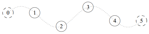
Figure \( 5.16\): \(n = 3\), \(A_{j}=\cos [(j-1 / 2) 3 \pi / 4] .\).

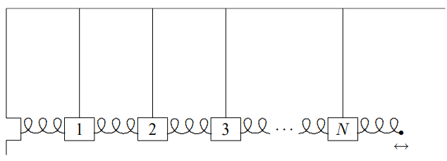
Figure \( 5.17\): A forced oscillation problem in a space translation invariant system.

This is the system of (5.1), except that one wall has been removed and the end of the spring is constrained by some external agency to move back and forth with a displacement \[z \cos \omega_{d} t .\]

As usual, in a forced oscillation problem, we first consider the driving term, in this case the fixed displacement of the \(N + 1\)st block, (5.49), to be the real part of a complex exponential driving term, \[z e^{-i \omega_{d} t} .\]

Then we look for a steady state solution in which the entire system is oscillating with the driving frequency \(\omega_{d}\), with the irreducible time dependence, \(e^{-i \omega_{d} t}\).

If there is damping from a frictional force, no matter how small, this will be the steady state solution that survives after all the free oscillations have decayed away. We can find such solutions by the same sort of trick that we used to find the modes of free oscillation of the system. We look for modes of the infinite system and put them together to satisfy boundary conditions.

This situation is different from the free oscillation problem. In a typical free oscillation problem, the boundary conditions fix \(k\). Then we determine \(\omega\) from the dispersion relation. In this case, the boundary conditions determine \(\omega_{d}\) instead. Now we must use the dispersion relation, (5.35), to find the wave number \(k\).

Solving (5.35) gives \[k=\frac{1}{a} \cos ^{-1} \frac{2 B-\omega_{d}^{2}}{2 C} .\]

We must combine the modes of the infinite system, \(e^{\pm i k x}\), to satisfy the boundary conditions at \(x = 0\) and \(x = (N + 1)a = L\). As for the system (5.1), the condition that the system be stationary at \(x = 0\) leads to a mode of the form \[\psi(x, t)=y \sin k x e^{-i \omega_{d} t}\]

for some amplitude \(y\). But now the condition at \(x = L = (N + 1)a\) determines not the wave number (that is already fixed by the dispersion relation), but the amplitude \(y\). \[\psi(L, t)=y \sin k L e^{-i \omega_{d} t}=z e^{-i \omega_{d} t} .\]

Thus \[y=\frac{z}{\sin k L} .\]

Notice that if \(\omega_{d}\) is a normal mode frequency of the system (5.1) with no damping, then (5.54) doesn’t make sense because \(\sin kL\) vanishes. That is as it should be. It corresponds to the infinite amplitude produced by a driving force on resonance with a normal frequency of a frictionless system. In the presence of damping, however, as we will discuss in chapter 8, the wave number \(k\) is complex because the dispersion relation is complex. We will see later that if \(k\) is complex, \(\sin kL\) cannot vanish. Even if the damping is very small, of course, we do not get a real infinity in the amplitude as we go to the resonance. Eventually, nonlinear effects take over. Whether it is nonlinearity or the damping that is more important near any given resonance depends on the details of the physical system.⁵

Forced Oscillations with a Free End

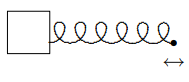
Figure \( 5.18\): Forced oscillation of a mass on a spring.

As another example, we will now discuss again the forced longitudinal oscillations of the simple system of a mass on a spring, shown in Figure \( 5.18\). The physics here is the same as that of the system in Figure \( 2.9\), except that to begin with, we will ignore damping. The block has mass \(m\). The spring has spring constant \(K\) and equilibrium length \(a\). To be specific, imagine that this block sits on a nearly frictionless table, and that you are holding onto the other end of the spring, moving it back and forth along the table, parallel to the direction of the spring, with displacement \[d_{0} \cos \omega_{d} t .\]

The question is, how does the block move? We already know how to solve this problem from chapter 2. Now we will do it in a different way, using space translation invariance, local interactions and boundary conditions. It may seem surprising that we can treat this problem using the techniques we have developed to deal with space translation invariant systems, because there is only one block. Nevertheless, that is what we are going to do. Certainly nothing prevents us from extending this system to an infinite system by repeating the block-spring combination. The infinite system then has the dispersion relation of the beaded string (or of the coupled pendulum for \(\ell \rightarrow \infty\)): \[\omega_{d}^{2}=\frac{4 K}{m} \sin ^{2} \frac{k a}{2} .\]

The relevant part of the infinite system is shown in Figure \( 5.19\). The point is that we can impose boundary conditions on the infinite system, Figure \( 5.19\), that make it equivalent to Figure \( 5.18\).

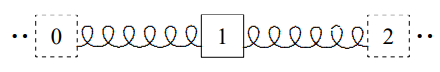
Figure \( 5.19\): Part of the infinite system.

We begin by imagining that the displacement is complex, \(d_{0} e^{-i \omega_{d} t}\), so that at the end, we will take the real part to recover the real result of (5.55). Thus, we take \[\psi_{2}(t)=d_{0} e^{-i \omega_{d} t} .\]

Then to ensure that there is no force on block 1 from the imaginary spring on the left, we must take \[\psi_{0}(t)=\psi_{1}(t) .\]

To satisfy (5.58), we can argue as in Figure \( 5.13\) that \[\psi(x, t)=z(t) \cos k x\]

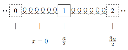
Figure \( 5.20\): A better definition of the zero of \(x\).

where \(x\) is defined as shown in Figure \( 5.20\).

Now since the equilibrium position of block 2 is \(3 a / 2\), we substitute \[\psi_{2}(t)=z(t) \cos \frac{3 k a}{2}\]

into (5.57), to obtain \[z(t)=\frac{d_{0}}{\cos \frac{3 k a}{2}} e^{-i \omega_{d} t} .\]

Then the final result is \[\psi_{1}(t)=\frac{\cos \frac{k a}{2}}{\cos \frac{3 k a}{2}} d_{0} e^{-i \omega_{d} t}\]

or in real form \[\psi_{1}(l)=\frac{\cos \frac{k a}{2}}{\cos \frac{3 k a}{2}} d_{0} \cos \omega_{d} l .\]

We can now use the dispersion relation. First use trigonometry, \[\cos 3 y=\cos ^{3} y-3 \cos y \sin ^{2} y=\cos y\left(1-4 \sin ^{2} y\right)\]

to write \[\psi_{1}(t)=\frac{1}{1-4 \sin ^{2} \frac{k a}{2}} d_{0} \cos \omega_{d} t\]

or substituting (5.56), \[\psi_{1}(t)=\frac{\omega_{0}^{2}}{\omega_{0}^{2}-\omega_{d}^{2}} d_{0} \cos \omega_{d} t ,\]

where \(\omega_{0}\) is the free oscillation frequency of the system, \[\omega_{0}^{2}=\frac{K}{m} .\]

This is exactly the same resonance formula that we got in chapter 2.

Generalization

The real advantage of the procedure we used to solve this problem is that it is easy to generalize it. For example, suppose we look at the system shown in Figure \( 5.21\).

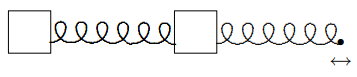
Figure \( 5.21\): A system with two blocks.

Here we can go to the same infinite system and argue that the solution is proportional to \(\cos kx\) where \(x\) is defined as shown in Figure \( 5.22\). Then the same argument leads to the result for the displacements of blocks 1 and 2: \[\psi_{1}(t)=\frac{\cos \frac{k a}{2}}{\cos \frac{5 k a}{2}} d_{0} \cos \omega_{d} t, \quad \psi_{2}(t)=\frac{\cos \frac{3 k a}{2}}{\cos \frac{5 k a}{2}} d_{0} \cos \omega_{d} t .\]

You should be able to generalize this to arbitrary numbers of blocks.

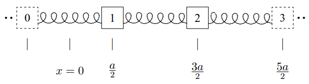
Figure \( 5.22\): The infinite system.

_____________________
⁵Note also that, when \(\sin kL\) is complex, the parts of the system do not all oscillate in phase, even though all oscillate at the same frequency.