5.3: Waves

Beaded String

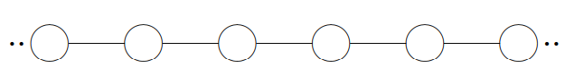
Figure \( 5.4\): The beaded string in equilibrium.

Another instructive system is the beaded string, undergoing transverse oscillations. The oscillations are called “transverse” if the motion is perpendicular to the direction in which the system is stretched. Consider a massless string with tension \(T\), to which identical beads of mass \(m\) are attached at regular intervals, \(a\). A portion of such a system in its equilibrium configuration is depicted in Figure \( 5.4\). The beads cannot oscillate longitudinally, because the string would break.³ However, for small transverse oscillations, the stretching of the string is negligible, and the tension and the horizontal component of the force from the string are approximately constant. The horizontal component of the force on each block from the string on its right is canceled by the horizontal component from the string on the left. The total horizontal force on each block is zero (this must be, because the blocks do not move horizontally). But the strings produces a transverse restoring force when neighboring beads do not have the same transverse displacement, as illustrated in Figure \( 5.5\). The force of the string on bead 1 is shown, along with the transverse component. The dotted lines complete similar triangles, so that \(F / T=\left(\psi_{2}-\psi_{1}\right) / a\). You can see from Figure \( 5.5\) that the restoring force, \(F\) in the figure, for small transverse oscillations is linear, and corresponds to a spring constant \(T / a\).

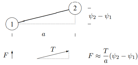
Figure \( 5.5\): Two neighboring beads on a beaded string.

Thus (5.37) is also the dispersion relation for the small transverse oscillations of the beaded string with \[B=\frac{T}{m a},\]

where \(T\) is the string tension, \(m\) is the bead mass and \(a\) is the separation between beads. The dispersion relation for the beaded string can thus be written as \[\omega^{2}=\frac{4 T}{m a} \sin ^{2} \frac{k a}{2}\]

This dispersion relation, (5.39), has the interesting property that \(\omega \rightarrow 0\) as \(k \rightarrow 0\). This is discussed from the point of view of symmetry in appendix C, where we discuss the connection of this dispersion relation with what are called “Goldstone bosons.” Here we should discuss the special properties of the \(k = 0\) mode with exactly zero angular frequency, \(\omega = 0\). This is different from all other angular frequencies because we do not get a different time dependence by complex conjugating the irreducible complex exponential, \(e^{-i \omega t}\). But we need two solutions in order to describe the possible initial conditions of the system, because we can specify both a displacement and a velocity for each bead. The resolution of this dilemma is similar to that discussed for critical damping in chapter 2 (see (2.12)). If we approach \(\omega = 0\) from nonzero \(\omega\), we can form two independent solutions as follows:⁴ \[\lim _{\omega \rightarrow 0} \frac{e^{-i \omega t}+e^{i \omega t}}{2}=1, \quad \lim _{\omega \rightarrow 0} \frac{e^{-i \omega t}-e^{i \omega t}}{-2 i \omega}=t\]

The first, for \(k = 0\), describes a situation in which all the beads are sitting at some fixed position. The second describes a situation in which all of the beads are moving together at constant velocity in the transverse direction.

Precisely analogous things can be said about the \(x\) dependence of the \(k = 0\) mode. Again, approaching \(k = 0\) from nonzero \(k\), we can form two modes, \[\lim _{k \rightarrow 0} \frac{e^{i k x}+e^{-i k x}}{2}=1, \quad \lim _{k \rightarrow 0} \frac{e^{i k x}-e^{-i k x}}{2 i k}=x\]

The second mode here describes a situation in which each subsequent bead is more displaced. The transverse force on each bead from the string on the left is canceled by the force from the string on the right.

Fixed Ends

5-2

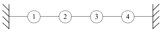
Figure \( 5.6\): A beaded string with fixed ends.

Now suppose that we look at a finite beaded string with its ends fixed at \(x = 0\) and \(x = L = (N + 1)a\), as shown in Figure \( 5.6\). The analysis of the normal modes of this system is exactly the same as for the coupled pendulum problem at the beginning of the chapter. Once again, we imagine that the finite system is part of an infinite system with space translation invariance and look for linear combinations of modes such that the beads at \(x = 0\) and \(x = L\) are fixed. Again this leads to (5.33). The only differences are:

1. the frequencies of the modes are different because the dispersion relation is now given by (5.39);
2. (5.33) describes the transverse displacements of the beads.

This is a very nice example of the standing wave normal modes, (5.33), because you can see the shapes more easily than for longitudinal oscillations. For four beads (\(N = 4\)), the four independent normal modes are illustrated in \(Figures \text { } 5.7 \text {-} 5.10\), where we have made the coupling strings invisible for clarity. The fixed imaginary beads that play the role of the walls are shown (dashed) at \(x = 0\) and \(x = L\). Superimposed on the positions of the beads is the continuous function, \(\sin k x\), for each \(k\) value, represented by a dotted line. Note that this function does not describe the positions of the coupling strings, which are stretched straight between neighboring beads.

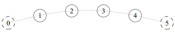
Figure \( 5.7\): \(n = 1\).

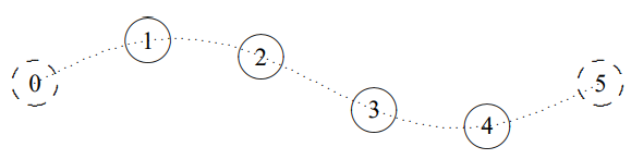
Figure \( 5.8\): \(n = 2\).

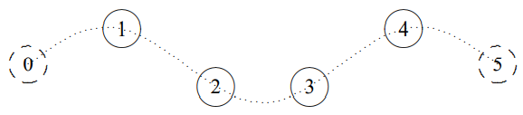
Figure \( 5.9\): \(n = 3\).

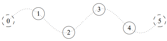
Figure \( 5.10\): \(n = 4\).

It is pictures like \(Figures \text { } 5.7 \text {-} 5.10\) that justify the word “wave” for these standing wave solutions. They are, frankly, wavy, exhibiting the sinusoidal space dependence that is the sine qua non of wave phenomena.

The transverse oscillation of a beaded string with both ends fixed is illustrated in program 5-2, where a general oscillation is shown along with the normal modes out of which it is built. Note the different frequencies of the different normal modes, with the frequency increasing as the modes get more wavy. We will often use the beaded string as an illustrative example because the modes are so easy to visualize.

_________________________
³More precisely, the string has a very large and nonlinear force constant for longitudinal stretching. The longitudinal oscillations have a much higher frequency and are much more strongly damped than the transverse oscillations, so we can ignore them in the frequency range of the transverse modes. See the discussion of the “light” massive spring in chapter 7.
⁴You can evaluate the limits easily, using the Taylor series for \(e^{x}=1+x+\cdots\).