5.4: Free Ends

Let us work out an example of forced oscillation with a different kind of boundary condition. Consider the transverse oscillations of a beaded string. For definiteness, we will take four beads so that this is a system of four coupled oscillators. However, instead of coupling the strings at the ends to fixed walls, we will attach them to massless rings that are free to slide in the transverse direction on frictionless rods. The string then is said to have its ends free (at least for transverse motion). Then the system looks like the diagram in Figure \( 5.11\), where the oscillators move up and down in the plane of the paper: Let us find its normal modes.

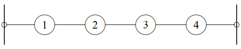
Figure 5.11: A beaded string with free ends.

Normal Modes for Free Ends

5-3
As before, we imagine that this is part of an infinite system of beads with space translation invariance. This is shown in Figure \( 5.12\). Here, the massless rings sliding on frictionless rods have been replaced by the imaginary (dashed) beads, 0 and 5. The dispersion relation is just the same as for any other infinite beaded string, (5.39). The question is, then, what kind of boundary condition on the infinite system corresponds to the physical boundary condition, that the end beads are free on one side? The answer is that we must have the first imaginary bead on either side move up and down with the last real bead, so that the coupling string from bead 0 is horizontal and exerts no transverse restoring force on bead 1 and the coupling string from bead 5 is horizontal and exerts no transverse restoring force on bead 4: \[A_{0}=A_{1} ,\]

\[A_{4}=A_{5} ;\]

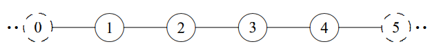
Figure \( 5.12\): Satisfying the boundary conditions in the finite system.

We will work in the notation in which the beads are labeled by their equilibrium positions. The normal modes of the infinite system are then \(e^{\pm i k x}\). But we haven’t yet had to decide where we will put the origin. How do we form a linear combination of the complex exponential modes, \(e^{\pm i k x}\), and choose \(k\) to be consistent with this boundary condition? Let us begin with (5.42). We can write the linear combination, whatever it is, in the form \[\cos (k x-\theta) .\]

Any real linear combination of \(e^{\pm i k x}\) can be written in this way up to an overall multiplicative constant (see (1.96)). Now if \[\cos \left(k x_{0}-\theta\right)=\cos \left(k x_{1}-\theta\right) ,\]

where \(x_{j}\) is the position of the \(j\)th block, then either

1. \(\cos (k x-\theta)\) has a maximum or minimum at \(\frac{x_{0}+x_{1}}{2}\), or
2. \(k x_{1}-k x_{0}\) is a multiple of \(2 \pi\).

Let us consider case 1. We will see that case 2 does not give any additional modes. We will \(\frac{x_{0}+x_{1}}{2}\) choose our coordinates so that the point , midway between \(x_{0}\) and \(x_{1}\), is \(x = 0\). We don’t care about the overall normalization, so if the function has a minimum there, we will multiply it by −1, to make it a maximum. Thus in case 1, the function \(\cos (k x-\theta)\) has a maximum at \(x = 0\), which implies that we can take \(\theta = 0\). Thus the function is simply \(\cos kx\). The system with this labeling is shown in Figure \( 5.13\). The displacement of the \(j\)th bead is then \[A_{j}=\cos [k a(j-1 / 2)] .\]

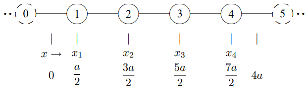
Figure \( 5.13\): The same system of oscillators labeled more cleverly.

It should now be clear how to impose the boundary condition, (5.43), on the other end. We want to have a maximum or minimum midway between bead 4 and bead 5, at \(x = 4a\). We get a maximum or minimum every time the argument of the cosine is an integral multiple of \(\pi\). The argument of the cosine at \(x = 4a\) is \(4ka\), where \(k\) is the angular wave number. Thus the boundary condition will be satisfied if the mode has \(4ka = n \pi\) for integer \(n\). Then \[\cos [k a(4-1 / 2)]=\cos [k a(5-1 / 2)] \Rightarrow k a=\frac{n \pi}{4} .\]

Thus the modes are \[A_{j}=\cos [k a(j-1 / 2)] \text { with } k=\frac{n \pi}{4 a} \text { for } n=0 \text { to } 3 .\]

For \(n > 3\), the modes just repeat, because \(k \geq \pi / a\).

In (5.48), \(n = 0\) is the trivial mode in which all the beads move up and down together. This is possible because there is no restoring force at all when all the beads move together. As discussed above (see (5.40)) the beads can all move with a constant velocity because \(\omega = 0\) for this mode. Note that case 2, above, gives the same mode, and nothing else, because if \(k x_{1}-k x_{0}=2 n \pi\), then (5.44) has the same value for all \(x_{j}\). The remaining modes are shown in \(Figures \text { } 5.14 \text{-} 5.16\). This system is illustrated in program 5-3 on the program disk.

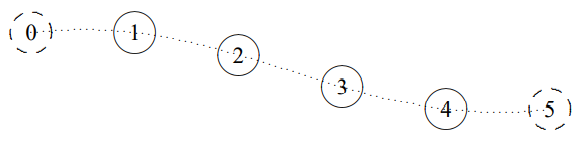
Figure \( 5.14\): \(n = 1\), \(A_{j}=\cos [(j-1 / 2) \pi / 4]\).

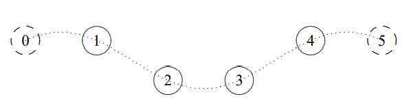
Figure \( 5.15\): \(n = 2\), \(A_{j}=\cos [(j-1 / 2) 2 \pi / 4]\).