5.6: Coupled LC Circuits

We saw in chapter 1 the analogy between the \(LC\) circuit in Figure \( 1.10\) and a corresponding system of a mass and springs in Figure \( 1.11\). In this section, we discuss what happens when we put \(LC\) circuits together into a space translation invariant system.

For example, consider an infinite space translation invariant circuit, a piece of which is shown in Figure \( 5.23\). One might guess, on the basis of the discussion in chapter 1, that the circuit in Figure \( 5.23\) is analogous to the combination of springs and masses shown in

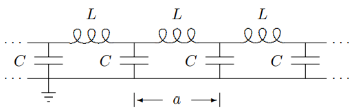
Figure \( 5.23\): A an infinite system of coupled \(LC\) circuits.

Figure \( 5.24\), with the correspondence between the two systems being: \[\begin{aligned}
m & \leftrightarrow \quad L \\
K & \leftrightarrow 1 / C \\
x_{j} & \leftrightarrow \quad Q_{j}
\end{aligned}\]

where \(x_{j}\) is the displacement of the \(j\)th block to the right and \(Q_{j}\) is the charge that has been “displaced” through the \(j\)th inductor from the equilibrium situation with the capacitors uncharged. In fact, this is right, and we could use (5.69) to write down the dispersion relation for the Figure \( 5.23\). However, with our powerful tools of linearity and space translation invariance, we can solve the problem from scratch without too much effort. The strategy will be to write down what we know the solution has to look like, from space translation invariance, and then work backwards to find the dispersion relation.

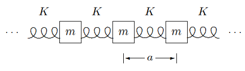
Figure \( 5.24\): A mechanical system analogous to Figure \( 5.23\).

The starting point should be familiar by now. Because the system is linear and space translation invariant, the modes of the infinite system are proportional to \(e^{\pm i k x}\). Therefore all physical quantities in a mode, voltages, charges, currents, whatever, must also be proportional to \(e^{\pm i k x}\). In this case the variable, \(x\), is really just a label. The electrical properties of the circuit do not depend very much on the disposition of the elements in space.⁶ The dispersion relation will depend only on \(ka\), where \(a\) is the separation between the identical parts of the system (see (5.35)). However, it is easier to think about the system if it is physically laid out into a space translation invariant configuration, as shown in Figure \( 5.23\).

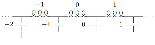
Figure \( 5.25\): A labeling for the infinite system of coupled \(LC\) circuits.

In particular, let us label the inductors and capacitors as shown in Figure \( 5.25\). Then the charge displaced through the \(j\)th inductor in the mode with angular wave number, \(k\), is \[Q_{j}(t)=q e^{i j k a} e^{-i \omega t}\]

for some constant charge, \(q\). Note that we could just as well take the time dependence to be \(\cos \omega t\), \(\sin \omega t\), or \(e^{i \omega t\). It does not matter for the argument below. What matters is that when we differentiate \(Q_{j}(t)\) twice with respect to time, we get \(-\omega^{2} Q_{j}(t)\). The current through the \(j\)th inductor is \[I_{j}=\frac{d}{d t} Q_{j}(t)=-i \omega q e^{i j k a} e^{-i \omega t} .\]

The charge on the \(j\)th capacitor, which we will call \(q_{j}\), is also proportional to \(e^{i j k a} e^{-i \omega t}\), but in fact, we can also compute it directly. The charge, \(q_{j}\), is just \[q_{j}=Q_{j}-Q_{j+1}\]

because the charge displaced through the \(j\)th inductor must either flow onto the \(j\)th capacitor or be displaced through the \(j + 1\)st inductor, so that \(Q_{j}=q_{j}+Q_{j+1}\). Now we can compute the voltage, \(V_{j}\), of each capacitor, \[V_{j}=\frac{1}{C}\left(Q_{j}-Q_{j+1}\right)=\frac{q}{C}\left(1-e^{i k a}\right) e^{i j k a} e^{-i \omega t} ,\]

and then compute the voltage drop across the inductors, \[L \frac{d I_{j}}{d t}=V_{j-1}-V_{j} ,\]

inserting (5.71) and (5.73) into (5.74), and dividing both sides by the common factor \(-q L e^{i j k a} e^{-i \omega t}\), we get the dispersion relation, \[\omega^{2}=-\frac{1}{L C}\left(1-e^{i k a}\right)\left(e^{-i k a}-1\right)=\frac{4}{L C} \sin ^{2} \frac{k a}{2} .\]

This corresponds to (5.37) with \(B = 1 / LC\). This is just what we expect from (5.69). We will call (5.75) the dispersion relation for coupled \(LC\) circuits.

Example of Coupled \(LC\) Circuits

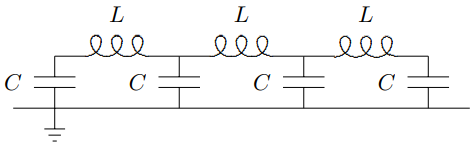
Figure \( 5.26\): A circuit with three inductors.

Let us use the results of this section to study a finite example, with boundary conditions. Consider the circuit shown in Figure \( 5.26\). This circuit in Figure \( 5.26\) is analogous to the combination of springs and masses shown in Figure \( 5.27\).

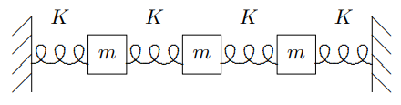
Figure \( 5.27\): A mechanical system analogous to Figure \( 5.26\).

We already know that this is true for the middle. It remains only to understand the boundary conditions at the ends. If we label the inductors as shown in Figure \( 5.28\), then we can imagine that this system is part of the infinite system shown in Figure \( 5.23\), with the charges constrained to satisfy \[Q_{0}=Q_{4}=0 .\]

This must be right. No charge can be displaced through inductors 0 and 4, because in Figure \( 5.26\), they do not exist. This is just what we expect from the analogy to the system in (5.27), where the displacement of the 0 and 4 blocks must vanish, because they are taking the place of the fixed walls.

Now we can immediately write down the solution for the normal modes, in analogy with (5.21) and (5.22), \[Q_{j} \propto \sin \frac{j n}{4}\]

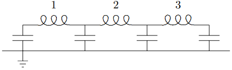
Figure \( 5.28\): A labeling of the inductors in Figure \( 5.26\).

for \(n\) = 1 to 3.

Forced Oscillation Problem for Coupled \(LC\) Circuits

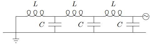
Figure \( 5.29\): A forced oscillation with three inductors.

One more somewhat more practical example may be instructive. Consider the circuit shown in Figure \( 5.29\). The in Figure \( 5.29\) stands for a source of harmonically varying voltage. We will assume that the voltage at this point in the circuit is fixed by the source, , to be \[V \cos \omega t .\]

We would like to find the voltages at the other nodes of the system, as shown in Figure \( 5.30\), with \[V_{3}-V \cos \omega t .\]

We could solve this problem using the displaced charges, however, it is a little easier to use the fact that all the physical quantities in the infinite system in Figure \( 5.23\) are proportional to \(e^{i k x}\) in a mode with angular wave number \(k\). Because this is a forced oscillation problem (and because, as usual, we are ignoring possible free oscillations of the system and looking for the steady state solution), \(k\) is determined from \(\omega\), by the dispersion relation for the infinite system of coupled \(LC\) circuits, (5.75).

The other thing we need is that \[V_{0}=0 ,\]

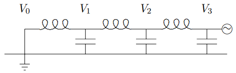
Figure \( 5.30\): The voltages in the system of Figure \( 5.29\).

because the circuit is shorted out at the end. Thus we must combine the two modes of the infinite system, \(e^{\pm i k x}\), into \(\sin kx\), and the solution has the form \[V_{j} \propto \sin j k a .\]

We can satisfy the boundary condition at the other end by taking \[V_{j}=\frac{V}{\sin 3 k a} \sin j k a \cos \omega t .\]

This is the solution.

_____________________
⁶This is not exactly true, however. Relativity imposes constraints. See chapter 11.