5.2: k and Dispersion Relations

So far, the equilibrium separation between the blocks, \(a\), has not appeared in the analysis. Everything we have said so far would be true even if the springs had random lengths, so long as all spring constants were the same. In such a case, the “space translation invariance” that we used to solve the problem would be a purely mathematical device, taking the original system into a different system with the same kind of small oscillations. Usually, however, in physical applications, the space translation invariance is real and all the inter-block distances are the same. Then it is very useful to label the blocks by their equilibrium position. Take \(x = 0\) to be the position of the left wall (or the 0th block). Then the first block is at \(x = a\), the second at \(x = 2a\), etc., as shown in Figure \( 5.3\). We can describe the displacement of all the blocks by a function \(\psi(x, t)\), where \(\psi(ja, t)\) is the displacement of the \(j\)th block (the one with equilibrium position \(ja\)). Of course, this function is not very well defined because we only care about its values at a discrete set of points. Nevertheless, as we will see below when we discuss the beaded string, it will help us understand what is going on if we draw a smooth curve through these points.

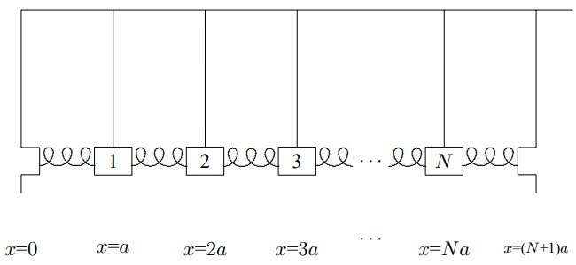
Figure \( 5.3\): The coupled pendulums with blocks labeled by their equilibrium positions.

In the same way, we can describe a normal mode of the system shown in Figure \( 5.1\) (or the infinite system of Figure \( 5.2\)) as a function \(A(x)\) where \[A(j a)=A_{j} .\]

In this language, space translation invariance, (5.11), becomes \[A(x+a)=\beta A(x) .\]

It is conventional to write the constant \(\beta\) as an exponential \[\beta=e^{i k a} .\]

Any nonzero complex number can be written as a exponential in this way. In fact, we can change \(k\) by a multiple of \(2 \pi / a\) without changing \(\beta\), thus we can choose the real part of \(k\) to be between \(- \pi / a\) and \(\pi / a\) \[-\frac{\pi}{a}<\operatorname{Re} k \leq \frac{\pi}{a} .\]

If we put (5.13) and (5.27) into (5.25), we get \[A^{\beta}(j a)=e^{i k j a} .\]

This suggests that we take the function describing the normal mode corresponding to (5.27) to be \[A(x)=e^{i k x} .\]

The mode is determined by the number \(k\) satisfying (5.28).

The parameter \(k\) (when it is real) is called the angular wave number of the mode. It measures the waviness of the normal mode, in radians per unit distance. The “wavelength” of the mode is the smallest length, \(\lambda\) (the Greek letter lambda), such that a change of \(x\) by \(\lambda\) leaves the mode unchanged, \[A(x+\lambda)=A(x) .\]

In other words, the wavelength is the length of a complete cycle of the wave, \(2 \pi\) radians. Thus the wavelength, \(\lambda\), and the angular wave number, \(k\), are inversely related, with a factor of \(2 \pi\), \[\lambda=\frac{2 \pi}{k} \text { . }\]

In this language, the normal modes of the system shown in Figure \( 5.1\) are described by the functions \[A^{n}(x)=\sin k x ,\]

with \[k=\frac{n \pi}{L} ,\]

where \(L = (N +1)a\) is the total length of the system. The important thing about (5.33) and (5.34) is that they do not depend on the details of the system. They do not even depend on \(N\). The normal modes always have the same shape, when the system has length \(L\). Of course, as \(N\) increases, the number of modes increases. For fixed L, this happens because \(a = L/(N + 1)\) decreases as \(N\) increases and thus the allowed range of \(k\) (remember (5.28)) increases.

The forms (5.33) for the normal modes of the space translation invariant system are called “standing waves.” We will see in more detail below why the word “wave” is appropriate. The word “standing” refers to the fact that while the waves are changing with time, they do not appear to be moving in the \(x\) direction, unlike the “traveling waves” that we will discuss in chapter 8 and beyond.

Dispersion Relation

In terms of the angular wave number \(k\), the frequency of the mode is (from (5.16) and (5.27)) \[\omega^{2}=2 B-2 C \cos k a .\]

Such a relation between \(k\) (actually \(k^{2}\) because \(\cos k a\) is an even function of \(k\)) and \(\omega^{2}\) is called a “dispersion relation” (we will learn later why the name is appropriate). The specific form (5.35) is a characteristic of the particular infinite system of Figure \( 5.2\). It depends on the masses and spring constants and pendulum lengths and separations.

But it does not depend on the boundary conditions. Indeed, we will see below that (5.35) will be useful for boundary conditions very different from those of the system shown in Figure \( 5.1\).

The dispersion relation depends only on the physics of the infinite system.

Indeed, it is only through the dispersion relation that the details of the physics of the infinite system enters the problem. The form of the modes, \(e^{\pm i k x}\), is already determined by the general properties of linearity and space translation invariance.

We will call (5.35) the dispersion relation for coupled pendulums. We have given it a special name because we will return to it many times in what follows. The essential physics is that there are two sources of restoring force: gravity, that tends to keep all the masses in equilibrium; and the coupling springs, that tend to keep the separations between the masses fixed, but are unaffected if all the masses are displaced by the same distance. In (5.35), the constants always satisfy \(B \geq C\), as you see from (5.6).

The limit \(B = C\) is especially interesting. This happens when there is no gravity (or \(\ell \rightarrow \infty\)). The dispersion relation is then \[\omega^{2}=2 B(1-\cos k a)=4 B \sin ^{2} \frac{k a}{2} .\]

Note that the mode with \(k = 0\) now has zero frequency, because all the masses can be displaced at once with no restoring force.²

_______________________
²See appendix \(C\).