3.3: Electric Potential Energy

Learning Objectives

By the end of this section, you will be able to:

• Define the work done by an electric force.
• Define electric potential energy.
• Apply work and potential energy in a system of a point charge in uniform electric field.

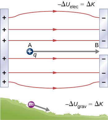
In this section, we begin to explore the use of energy to describe physical systems with electric charges through the definition of electric potential energy. Suppose a positively-charged particle is placed in between a positive plate and another equally-charged, parallel negative plate (Figure \(\PageIndex{1}\)). From Common Electric Field Models, we know that a nearly uniform electric field will exist between the plates directed from the positive plate to the negative plate. From Electric Fields and Forces, we also know that the electric field will exert a force on the positive charge in the same direction as the field. When the free positive charge \(q\) is accelerated by an electric field, it gains kinetic energy. The process is analogous to an object being accelerated by a gravitational field, as if the charge were going down an electrical hill where its electric potential energy is converted into kinetic energy, although, of course, the sources of the forces are very different. Let us explore the work done on a charge \(q\) by the electric field in this process, so that we may develop a definition of electric potential energy.

Figure \(\PageIndex{1}\): A charge accelerated by an electric field is analogous to a mass going down a hill. In both cases, potential energy decreases as kinetic energy increases, \(-\Delta U = \Delta K\). Work is done by a force, but since this force is conservative, we can write \(W = -\Delta U\).

As we will demonstrate later, the electric force is a conservative force, which means that the work done on \(q\) is independent of the path taken. This is exactly analogous to the gravitational force. When a force is conservative, it is possible to define a potential energy associated with the force. It is usually easier to work with the potential energy (because it depends only on position) than to calculate the work directly.

Example \(\PageIndex{1}\) shows how the gravitational potential energy can be calculated for the analogous system of a mass in a gravitational field.

Example \(\PageIndex{1}\)

What is the gravitational potential energy of a mass \(m\) at a height \( y\) above the ground near the surface of the Earth?

Solution

From the example in Electric Fields and Forces, we know how to calculate the gravitational force on a mass from the nearly-constant gravitational field near the surface of the Earth. From the expression for work in Work and Energy, we can then calculate the work done on the mass by the gravitational force as the mass falls from an initial height to its final height. Because we know the gravitational force is a conservative force, we can then relate the work done on the mass to the change in the gravitational potential energy in the system.

Figure \(\PageIndex{2}\) shows a diagram of the system, including the gravitational field and gravitational force, in its initial state and then, after it has fallen, in its final state. Observe that the displacement is parallel to the gravitational force.

Figure \(\PageIndex{2}\): Initial and final states of a mass falling in a gravitational field. [1]

CALCULATE

The gravitational force on the mass is \(\vec{F}=m\vec{g}= mg (-\hat{j})\). The work done by the gravitational force on the mass during its displacement  \( \Delta\vec{r} = (y_i - y_f) (-\hat{j}) \) is then

\[ W = \vec{F}\cdot\Delta\vec{r} = |\vec{F}| |\Delta \vec{r}| \cos 0^\circ = mg (y_i - y_f). \nonumber \]

For a conservative force, the change in the gravitational potential energy is

\[ \Delta U_G = -W = -mg(y_i - y_f) = mgy_f - mgy_i = U_f - U_i . \nonumber \]

Hence it follows that the gravitational potential energy

\[ U_G = mgy + U_0 , \label{PEgravity} \]

where \( U_0 \) is the value of the potential energy at the ground (\(y = 0\)). This value is arbitrary, and we choose to set it to zero for convenience. Only differences in energy are physically significant so adding a constant value will not affect the physical response of the system.

CHECK

We know from experience that the gravitational potential energy is greater at larger heights, which is consistent with the given result.

Observe that the parallel-charged plates create a uniform electric field much like the uniform gravitational field near the surface of the Earth. As a result, Example \(\PageIndex{2}\) shows that we can follow a similar analysis to find the electric potential energy of the system in Fig. \(\PageIndex{1}\).

Example \(\PageIndex{2}\)

What is the electrical potential energy of a charge \(q\) at a distance \( y \) away from the negative plate of the oppositely-charged parallel plates in Fig. \(\PageIndex{1}\)?

Solution

From Electric Fields and Forces, we know how to calculate the electric force on a charge. From the expression for work in Work and Energy, we then can calculate the work done on the charge by the electric force as the charge moves from its initial position to its final position. If we assume the electric force is a conservative force, we can then relate the work done on the charge to the change in the electrical potential energy in the system.

Figure \(\PageIndex{3}\) shows a diagram of the system, including the electric field and electric force, in its initial state and then, after the particle has moved, in its final state. Observe that the displacement is parallel to the electric force.

Figure \(\PageIndex{3}\): Initial and final states of a positive charge attracted to the negative plate in a set of oppositely-charged parallel plates. Each plate has an equal amount of charge. [2]

CALCULATE

The electric force on the charge is \(\vec{F}=q\vec{E}= qE (-\hat{j})\). The work done by the electric force on the charge during its displacement
\( \Delta\vec{r} = (y_i - y_f) (-\hat{j}) \) is then

\[ W = \vec{F}\cdot\Delta\vec{r} = |\vec{F}| |\Delta \vec{r}| \cos 0^\circ = qE (y_i - y_f). \nonumber \]

For a conservative force, the change in the gravitational potential energy is

\[ \Delta U_E = -W = -qE(y_i - y_f) = qEy_f - qEy_i = U_f - U_i . \nonumber \]

Hence it follows that the gravitational potential energy

\[ U_E = qEy + U_0 , \label{PEelectric} \ \ \ \ \ \text{(electric potential energy of point charge in a uniform field)} \]

where \( U_0 \) is the value of the potential energy at the ground (\(y = 0\)), which you could set to be zero, if you so choose. Note that while the figure shows a positive charge, all the steps in the calculation are still correct if the charge is negative.

CHECK

Equation \ref{PEelectric} shows that the electric potential energy is greater when the charge is further away from the negative plate. This result makes sense because the positive charge is attracted to the negative plate, and, thus, it will take work to push it away from the negative plate. Moreover, we know that the positive charge will accelerate toward the negative plate, thereby gaining kinetic energy. By conservation of energy, the increase in kinetic energy of the charge must come from a decrease in the electric potential energy of the charge as it moves toward the plate.

For the system in Fig. \(\PageIndex{1}\), we can construct an energy diagram (Fig. \(\PageIndex{1}\)). This energy diagram plots energy on the vertical axis and the distance from the negative plate on the horizontal axis. Given Equation \ref{PEelectric} with \(U_0 = 0\), the electric potential should be zero at the negative plate and then increase linearly away from the plate (recall that the positive y-axis is to the left). If a positively-charged particle is close to the negative plate and then is given a "kick" toward the positively charged plate, it will have a certain total amount of mechanical energy \(E_{mech}\). The difference between the total mechanical energy and electric potential energy \(U_E\) is then kinetic energy \(K\). However, the positive charge is repelled from the positive plate, and therefore should slow down. At some distance \(y_{max}\), the particle comes to a stop as the electric potential energy \(U_E = E_{mech}\) and therefore \(K = 0\). This position is called the turning point, as the particle will stop there, and then turn around and accelerate back toward the negative plate.

Figure \(\PageIndex{4}\): Energy diagram for a positively charged particle in between parallel plates with equal but opposite charge. [3]

Exercise \(\PageIndex{1}\)

How will the energy diagram change if the particle in between the charged plates of Fig. \(\PageIndex{1}\) is negative?

Answer

According to Equation \ref{PEelectric}, the potential energy will be still linear, but negatively-valued with its maximum at \(y=0\). As particles tend toward a lower energy state, this means that the particle will move to the left losing potential energy (becoming more negative) and gaining kinetic energy. This outcome is consistent with the force perspective because we expect that the negatively-charged particle will be attracted to the positive plate and will accelerate as it moves in that direction.

The electric potential energy of a charged particle in a uniform field is a good starting point for our discussion, but it is a special case. In the next section, we will consider the more general case of the electric potential energy of a point charge in the electric field created by other point charges.

References

1. Ronald E. Kumon. [Internet] GravitationalPotential.png. (CC-BY-SA 4.0)
2. Background Image: University Physics, Volume 2. OpenStax; 2021. Modifications by Ronald E. Kumon. [Internet] ElectricPotential_UniformField.png. (CC-BY-SA 4.0)
3. Background Image: University Physics, Volume 2. OpenStax; 2021. Modifications by Ronald E. Kumon. [Internet] ElectricPotential_UniformField.png. (CC-BY-SA 4.0)