7.5: Torque

Rotational Analog to Force

We have developed multiple analogs between linear and rotational motion so far: velocity, acceleration, kinetic energy, and mass. We have seen Newton's 2nd Law which relates force to mass and acceleration, which tells us how the linear motion of an object changes due to external forces. Now we want to develop the analog of the 2nd Law with will relate "rotational force", known as torque, \(\vec\tau\), which will determine how angular motion will change. There is a fundamental difference between force and torque as we will see shortly, specifically, not all forces will result in torques, and not all torques will results in net forces. Since rotational inertia is analogous to mass, and angular acceleration is analogous to linear acceleration, we can write down the analog of Newton's 2nd Law:

\[\vec a=\frac{\vec F}{m}~\Longleftrightarrow~\vec\alpha=\frac{\vec\tau}{I}\label{torque-Newton}\]

Torque is a vector since angular acceleration is a vector, and rotational inertia is a scalar. Let us examine which variables torque depends on by thinking about its units:

\[\tau=I\alpha=\Big[kg\cdot m^2\Big]\Big[\frac{\textrm{rad}}{s^2}\Big]=\Big[\frac{kg\cdot m^2}{s^2}\Big]=[N\cdot m]\label{units}\]

The last equality in the above equation comes from definition of Newtons: \(F=ma=[kg\cdot m/s^2]\equiv[N]\). So we find that torque will have units of force times length. Let's examine a simple example of a point mass attached to a massless rod of length \(r\) as shown in Figure 7.5.1. The rod is attached at a pivot on the opposite end of the mass.

Figure 7.5.1: Torque on a Point Mass

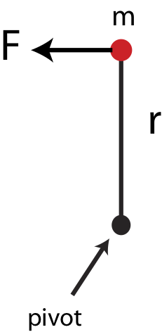
Focusing on magnitude only for now and applying Newton's 2nd Law for linear motion to the mass and using the connection between linear and angular acceleration, \(a=r\alpha\), we find that:

\[ F=ma=mr\alpha\]

For a point mass the rotational inertia from the pivot is \(I=mr^2\). Multiplying both sides of the equation above by \(r\) we get:

\[Fr=mr^2\alpha=I\alpha\]

Comparing the above result with Equation \ref{torque-Newton} we conclude that for a point mass:

\[\tau=rF\label{tau-Nm}\]

This result is consistent with the argument in Equation \ref{units} that torque has units of \(N\cdot m\). Although we demonstrated the result in Equation \ref{tau-Nm} specifically for a point mass, it turns out to be general for any set of masses or for an object with continuous mass, where \(r\) represents a distance from the pivot to the location where the force is applied. The result of torque being proportional to distance from pivot implies that the further the force is from the pivot, the bigger will be the torque, and the greater the angular acceleration. We have experienced this phenomena in many instances. For example, the pivot can represent a hinge of a door. The door swings back and forth about the hinge, and we apply forces to the door when we push it in order to open it. The further away from the door you push, the easier it is to open it since you are applying a greater torque simply by applying a force further from the hinge (pivot). We have all faced challenges of trying to open a heavy door by accidentally pushing it very close to the hinge.Our discussion on torque is not yet complete since we also need to consider the direction of torque and its dependence on the direction of force. Figure 7.5.2 below shows three different cases of a force acting on a point mass attached to a massless rod, which is fixed in place at the pivot on other end of the bar. In case one the force will result in an angular acceleration counterclockwise. In case 2 the acceleration will be in the clockwise direction. While in case 3 the rod will not rotate even if there is a force of the same magnitude acting on the mass.

Figure 7.5.2: Direction of Torque on a Point Mass

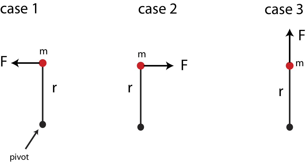
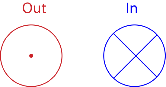
Thus, cases 1 and 2 generate a torque but in the opposite directions based on Equation \ref{torque-Newton}, while case 3 results in zero torque. For cases 1 and 2 we can use the same right hand rule as we did for angular velocity to determine the direction of torque. To use the RHR you point the fingers of your right hand from the pivot toward the force and then curl them in the direction of the force, which is the direction it which the object would rotate due to that force. Your thumb will point in the direction of torque. In case 1 this direction is out of the page, and for case 2 it is into the page. Since very often when discussing angular motion vectors will point either in or out of the page, we need symbols to represent these vectors, since we can no longer draw arrows in the two-dimensional space of the page. These symbols are shown below in Figure 7.5.4. The "out" vector show the head of an arrow pointing toward you, and the "in" vector shows the tail of the arrow which is sticking into the page. Unlike arrows drawn on the plane of the page which have a length and a direction, these vector symbols only demonstrate direction, since you cannot draw them as longer or shorter arrows. 

Figure 7.5.3: Vector Direction In and Out of the Page

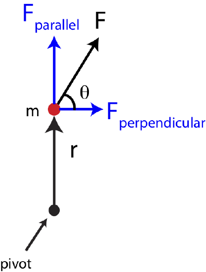
What we can conclude from the three cases in Figure 7.5.2 that whether a force generates a torques depends of its orientation relative to the pivot. We can define a force position vector, \(\vec r\), which points from the pivot or reference point to the location of the force. In Figure 7.5.2 we see that forces that are perpendicular to the position vector generate torque. On the contrary, forces that are parallel to the position vector, as in case 3, general zero torque. If a force was at an angle relative to the position vector, as shown in Figure 7.5.4, then it can be split into components parallel, \(F_{||}\), and perpendicular, \(F_{\perp}\) to \(\vec r\). Based on the argument of the three cases in Figure 7.5.2, only the perpendicular component of this force would contribute to torque.

Figure 7.5.4: Direction of Force and Torque

Equation \ref{tau-Nm} for a more general case of a force that has both a parallel and perpendicular component relative to the position vector is:

\[\tau=rF_{\perp}\label{tau-Fperp}\]

The equation above only give the magnitude of the torque, while the right-hand rule determines the direction. Mathematically, a cross product contains both the magnitude and direction of torque:

\[\vec\tau=\vec r\times\vec F\]

But in this class, we will typically use equation \ref{tau-Fperp} to calculate the torque, and the RHR to determine its direction.

Figure 7.5.5 shows the position vector \(\vec r\) drawn from the pivot to the location of the force, and then the perpendicular component of the force is depicted as \(F_{\perp}\). If we define the angle, \(\theta\) as the angle between the force vector and the position vector, then \(F_{\perp}=F\sin\theta\) and Equation \ref{tau-Fperp} becomes:

\[\tau=rF\sin\theta\label{tau-theta}\] 

Figure 7.5.5: Position Vector and Moment arm

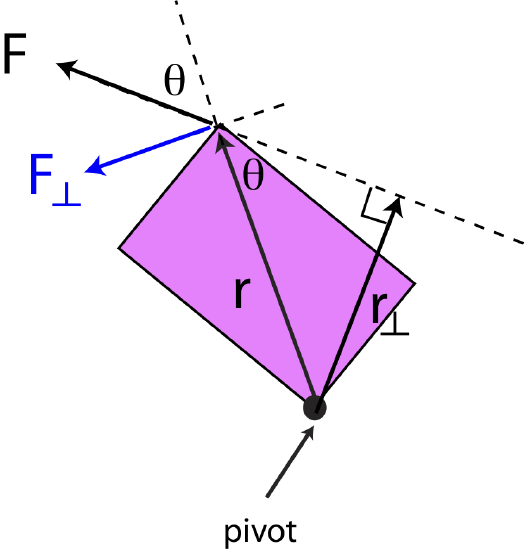
However, there are cases where using the position vector to calculate the magnitude of torque is not the simplest method geometrically. Thus, another method with the moment arm, \(r_{\perp}\), is sometimes used as shown in Figure 7.5.5. The vector \(r_{\perp}\) is drawn from the pivot point to the location where it is perpendicular to the force. Even if the force arrow is not physically there, we can extend it (dashed line extending the force vector in the figure) such that \(r_{\perp}\) is perpendicular to the line extending from the force. The two distances can be related by the same angle, \(\theta\) as:

\[r_{\perp}=r\sin\theta\]

Combing the above equation and Equation \ref{tau-theta}, the magnitude of torque can be written as:

\[\tau=r_{\perp}F\label{tau-rpepr}\]

The two methods described by Equations \ref{tau-Fperp} and \ref{tau-rpepr} give equivalent results. With practice you will find situations where one method is easier or quicker to use than another, depending on what is given and what needs to be calculated.

What we have learned by describing torque in this section so far is that the location of the force is essential in order to determine torque. Thus, when drawing a force diagram on a selected system, we can no longer collapse the extended object(s) into a point, which we did when calculating forces. For torque we need to draw the entire object and draw forces at the locations of their application. This is known as the extended force diagram, which needs to contain all the force vectors at their locations, the pivot or the point of reference from which torques are calculated, and all the distances marked from the pivot to each force. The extended force diagram contains all the information that a "collapsed" free-body diagram contains, so it can be used for calculating the net force as well as the net torque.

Example \(\PageIndex{1}\)

Shown below is a top view of a square shape anchored at the lower left corner with 5 forces acting on it. The length of each side of the square is 0.4 m. Forces 1-4 at at one of the corners of the square, while force 3 acts right at the center, as shown below. The magnitudes of the forces are given as:

\(F_1=F_2=5N, F_3=3N, F_4=2N,~\textrm{and}~F_5=7N\).

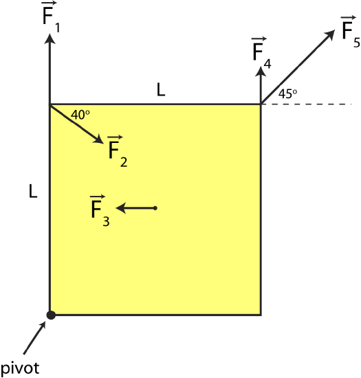
a) Calculate the net torque on the square. Express your answer in terms of magnitude and direction.

b) Calculate the net force on the square. Express your answer in terms of magnitude and direction.

Solution

a) The following diagram shows a convenient choice of using either position vector, \(\vec r\) or the moment arm \(r_{\perp}\) to solve for the torque due to each force.

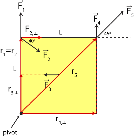
Force \(\vec F_1\) is parallel to the position vector \(\vec r_1\). Thus, there is no perpendicular component which results in zero torque due to this force:

\[\tau_1=0\nonumber\]

Force \(\vec F_2\) has the same position vector as \(\vec F_1\) (\(\vec r_2=\vec r_1\)), but there perpendicular component of this force to the position vector, \(F_{2,\perp}\):

\[F_{2,\perp}=F_2\cos 40^{\circ}=5N\cos 40^{\circ}=3.83~\textrm{N}\nonumber\]

The magnitude of the torque due to force 2 is then:

\[\tau_2=r_2F_{2,\perp}=(0.4m)(3.83N)=1.53~\textrm{Nm}\nonumber\]

Using the right hand-rule, fingers point up and curl toward \(F_{2,\perp}\) in the clockwise direction resulting in the thumb pointing into the page. Thus, the torque due to \(\vec F_1\) points into the page.

For \(\vec F_3\) it is simpler to use the moment arm method since you do not need to calculate any angles, as labeled in the figure \(r_{3,\perp}\). If you were to use the position vector, you would need to draw a vector pointing from the pivot to the location of \(\vec F_3\), and then calculate component of \(\vec F_3\) which is perpendicular to \(\vec r_3\). Also, you would need to calculate the length of \(\vec r_3\), which is half of the diagonal of the square. But using the moment arm gives a simple result to the magnitude of the torque due to force 3:

\[\tau_3=r_{3,\perp}F_3=\Big(\frac{0.4m}{2}\Big)(3N)=0.6~\textrm{Nm}\nonumber\]

Using RHR, we find that \(\vec F_3\) results in a clockwise rotation, so the torque point out of the page.

For \(\vec F_4\) it is again simpler to use the moment arm to calculate torque. Using \(r_{4,\perp}\) as marked in the figure we find:

\[\tau_4=r_{4,\perp}F_4=(0.4)(2N)=0.8~\textrm{Nm}\nonumber\]

Using RHR, we find that force 4 results in a clockwise rotation, so the torque point out of the page.

Force \(\vec F_5\) is parallel to the position vector, since \(\vec r_5\) makes exactly a \(45^{\circ}\) angle with the corner of the square, as does \(\vec F_5\). Since the two vectors are parallel there is no perpendicular component of the force to the position vector which results in zero torque: 

\[\tau_5=0\nonumber\]

Let us define a convention that vectors pointing out of the page are positive, and those pointing into the page are negative. Putting everything together the net torque is:

\[\vec\tau_{net}=\vec\tau_1+\vec\tau_2+\vec\tau_3+\vec\tau_4+\vec\tau_5=0-1.53+0.6+0.8+0=-0.13~\textrm{Nm}\nonumber\]

The magnitude of net torque is \(0.13~\textrm{Nm}\) and it point into the page.

b) To find the net force we need to break down the forces by components. In the x-direction:

\[F_{net,x}=F_{1,x}+F_{2,x}+F_{3,x}+F_{4,x}+F_{5,x}\nonumber\]

\[F_{net,x}=0+5N\cos 40^{\circ}-3N+0+7\cos 45^{\circ}=5.78~\textrm{N}\nonumber\]

In the y-direction:

\[F_{net,y}=F_{1,y}+F_{2,y}+F_{3,y}+F_{4,y}+F_{5,y}\nonumber\]

\[F_{net,y}=5N-5N\sin 40^{\circ}+0+2N+7\sin 45^{\circ}=8.74~\textrm{N}\nonumber\]

The magnitude is:

\[F_{net}=\sqrt{F_{net,x}^2+F_{net,y}^2}=\sqrt{5.78^2+8.74^2}=10.5~\textrm{N}\nonumber\]

And the angle is:

\[\theta=\arctan\Big(\frac{F_{net,y}}{F_{net,x}}\Big)=\arctan\Big(\frac{8.74}{5.78}\Big)=56.5^{\circ}\nonumber\]

pointing in the northeast direction.

 

The Center of Mass

You may have realized by now that modeling objects as point particles is a rather drastic oversimplification, even though it is often very useful. We have now seen instances when the extended geometry of a non-point object becomes important. Focusing on just one point of an object can describe perfectly adequately the translational motion of that object, but it does not tell us anything about the object’s rotation. It turns out that we can consider all of the forces acting on the object as if they acted at one point, the center of mass, as far as translation is concerned. That is, if we are concerned only about an object’s translation, it doesn’t matter where the forces act on the object. We can consider them all to act at a single point! This is truly a great simplification. The special point where we consider the forces to act is called the center of mass.

The center of mass is defined as a geometric average position of all the masses. For example, the center of mass of two point particles of equal mass is exactly at the midpoint between the two masses. If the masses are unequal, the center of mass would be closer to the heavier mass. Mathematically the center of mass can be described with an equation which expresses the average based on the relative weights of the masses. Figure 7.5.6 below shows a generalized system of two points masses, \(m_1\) and \(m_2\). The center of mass is the location measured relative to some arbitrary origin (x=0) along the line of the two masses. The distances marked \(x_1\) and \(x_2\) are the distances from the origin to each of the masses.

Figure 7.5.6: Center of Mass 

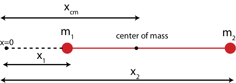
For the two masses shown in Figure 7.5.6, the center of mass is written as:

\[x_{cm}=\frac{m_1x_1+m_2x_2}{m_1+m_2}\]

From the equation we see that when \(m_1=m_2\) the center of mass becomes \(x_{cm}=(x_1+x_2)/2\) which is exactly the midpoint between the two masses. If \(m_1\gg m_2\), then the center of mass is very close to the location of \(m_1\), \(x_{cm}\sim x_1\). Extending this to a system of multiple number of point masses the center of mass equation becomes:

\[x_{cm}=\frac{\sum_{i=1}^{N}m_ix_i}{\sum_{i=1}^{N}m_i}=\frac{1}{M_{tot}}\sum_{i=1}^{N}m_ix_i\]

In nature most objects are not made up of a collection of point masses, but rather of a continuous mass. Mathematically, this means that we need to turn the summation to an integral over small mass elements, which can become rather complicated for an object in three-dimension with mass which is not uniform.

Torque due to Gravity

As we have just established in order to calculate torque on an object due to a force, you need to know the exact location where that force act. Gravity is a special case since it acts everywhere on a given object. And gravity can certainly cause torque, if you attempt hold a long and heavy stick at one end, it will want to rotate down due to torque cause by gravity. Thus, we want to figure out where to place the force of gravity on an extended object so we can calculate the amount of torque generated by gravity relative to some reference point.Consider the example in Figure 7.5.7 below, where a massless rod with two point masses at each end is balanced by a fulcrum, the pivot point where an object is balanced. The left picture shows an extended force diagram. Since the two masses are point masses, the force due to gravity on each mass is located exactly at the location of each mass.

Figure 7.5.7: Balanced Rod with Two Point Masses

 

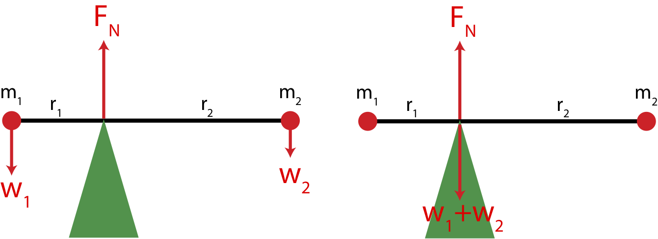
Relative to the fulcrum about which the rod pivots, the two weights generate torque in opposite directions. The right mass causes a torque into the page, while the left mass generates a torque out of the page. To balance torque, in addition to the direction being opposite, their magnitudes need to be the equal, \(\tau_1=\tau_2\). Using Equation \ref{tau-Fperp} we find that:

\[r_1m_1=r_2m_2\label{torque-balance}\]

Imagine that we did not have knowledge of the two point masses at the end of this rod, but instead just moved the fulcrum along the rod until it became balanced in this particular location. Since we now view this object as having some total mass (rather than a sum of two point masses) but with unknown distribution of that mass and there is no net torque once the fulcrum balances the object, the logical location of the weight of the object is at balance point. At the fulcrum which is the pivot, the position vector to the weight force is zero, so there is zero torque due to the weight. If we placed the weight vector anywhere other than the fulcrum, then it would generate a torque relative to the pivot, which is not consistent with the object being balanced. In other words, we can replace the two weights at the two point masses in the left picture with just one weight at the fulcrum of magnitude, \(w_1+w_2\), as shown in the right illustration. It turns out that this location is exactly at the center of mass of the object. You can see derivation of this fact below.

Derivation

We want to show that the result in Equation \ref{torque-balance} is exactly the center of mass of a two point particle system. Earlier in this section defined the center of mass of an object relative to some origin, as shown in the figure below.

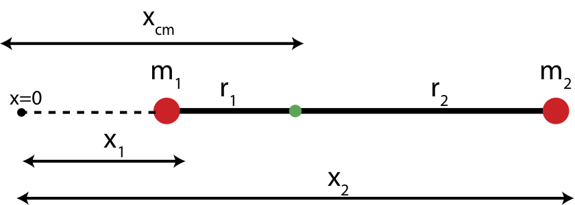
The center of mass relative to x=0 is given by:

\[x_{cm}=\frac{m_1x_1+m_2x_2}{m_1+m_2}\nonumber\]

We can rewrite \(r_1\) and \(r_2\) in terms of \(x_{cm}\) and \(x_1\) and \(x_2\). From the figure we see that:

\[r_1=x_{cm}-x_1\nonumber\]

and 

\[r_2=x_2-x_{cm}\nonumber\]

Plugging in the expression for \(x_{cm}\) into each equation we get:

\[r_1=\frac{m_1x_1+m_2x_2}{m_1+m_2}-x_1=\frac{m_2}{m_1+m_2}(x_2-x_1)\nonumber\]

and

\[r_2=x_2-\frac{m_1x_1+m_2x_2}{m_1+m_2}=\frac{m_1}{m_1+m_2}(x_2-x_1)\nonumber\]

Now let us multiple the equation for \(r_1\) by \(m_1\) and the equation for \(r_2\) by \(m_2\), and we see that the right hand sides of both equations becomes identical. So we can conclude that: 

\[r_1m_1=r_2m_2\nonumber\]

which is the exact equation that we obtained from balancing torque. Thus, the fulcrum was balanced at the center of mass of the two point object.

It turns out that the center of mass is the same as the center of gravity (where you can support the object and it will not rotate) as long as the gravitational force is uniform. Near the surface of the Earth, for all objects of ordinary size, the gravitational force can certainly be considered uniform. Thus, for all problems we consider, the center of mass and center of gravity are the same point.

If objects are constrained to rotate about a particular axis, such as a rod mounted by a hinge to a vertical wall the object is fixed at a specific location, the torques are typically computed about that axis. If there is no constraint, torques should be computed about the center of mass, the point about which the object will rotate. To see this, imagine you exert two forces of equal magnitude and opposite direction at different locations along the object. The different locations of force will result in a non-zero net torque, so the object will start rotating. Equal and opposite forces result in zero net force, so the center of mass cannot accelerate. If the object is rotating about the center of mass, it means that the center of mass is stationary, which is consistent with zero net force. If the object was rotating about any other reference point, that would imply that the center of mass is rotating about that point. In that case the velocity of the center of mass would be changing since its direction is changing, which can only happen if there is net force. Thus, the object must rotate about its center of mass.

Work

We are familiar with the concept of work as a way that the energy of a system is changed. In terms of force and distance, work is done to translate a system from position \(x_1\) to a new position \(x_2\) is given by:

\[W = \int \limits_{x_1}^{x_2} \overrightarrow F\cdot d\overrightarrow s\]

where the dot product of the two vectors reminds us that it is only the components of force and displacement in the same direction that contribute to the integral.

A similar expression holds for the work done by a torque to rotate a system from angle \(\theta_1\) to a new angle \(\theta_2\) is given by:

\[W =\int \limits_{\theta_1}^{\theta_2} \overrightarrow \tau\cdot d\overrightarrow {\theta}\]

The energy of a particular system can be changed by the process of a force exerted by an outside object doing work on an object in the system and/or by a torque exerted by an outside object doing work on an object within the system. In either case, the work can be positive (increases the energy of the system) or negative (decreases the energy of the system).