11.1: Fields

Introduction

A field is a concept that is used in almost every part of physics. In Physics 7C we will concentrate on the electric and magnetic fields. The concept of fields will help us understand how electric charges interact with each other and how those interactions lead to electric and magnetic forces. In the last section we will see electric and magnetic fields are closely related and can propagate: a phenomenon we commonly refer to as "light”! Thus, we will see that fields are not simply concepts that help us explain these interactions, but fields are indispensable: neglecting them would lead to a violation of both the conservation of energy and conservation of momentum. 

We will first start by discussing the potential energy that results from charges interacting, and see how that connects to electric forces. From this will will construct the potential field and the electric field, and develop the relationship between these fields and potential energy and the electric force. We will follow with the introduction of the magnetic field and magnetic force as we connect magnetism to electricity. 

The idea of a field is rooted in the concept that there is some physical quantity that has a value “everywhere". The value can either change from location to location or can stay the same. Both fields that vary in space and fields that are constant in (regions of) space are important. A field can vary in time as well as space, so any field that we discuss is a function of both position and time. While this is an easy thing to state, it is rather abstract, so let us become more familiar with this definition by looking at some examples of fields.

Scalar Fields

A scalar field is a field which describes a scalar quantity in space and time. The weather map below is similar to one you might see on the news: it represents a field. There is not one universal temperature, so you need to define both a time and a position where that temperature can be found. A question like “what is the temperature in San Francisco now?” can be answered because we have specified both the place and the time. In other words, the temperature \(T\) is a function of position \((x,y,z)\) (for example), and time \(t\).

Figure 11.1.1: Weather Map as a Scalar Field Representation 

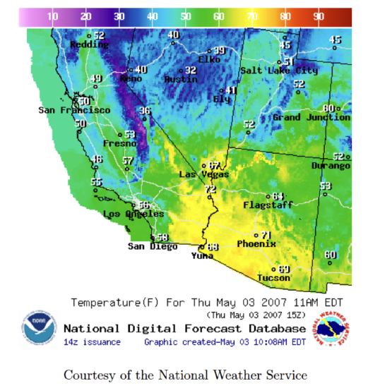
The weather map above is similar to one you might see on the news; it represents a field. There is not one universal temperature; the if you want to reference a temperature, you need to define both a time and a position where that temperature can be found. A question like “what is the temperature in San Francisco now?” can be answered because we have specified both the place and the time. In other words, the temperature \(T\) is a function of position \((x,y,z)\) (for example), and time \(t\).

With that being said, let's note a few important things about the map above:

• It shows temperatures at a particular time, so what is being shown is \(T(x, y, t = \text{today})\). The full field \(T(x, y, t)\) could be represented by an entire archive of all previous (and future!) temperature maps.
• On this map, the temperature is represented as a color, with the scale above giving the corresponding values.
• On some weather maps the temperature is only shown for selected locations. Even in the places where a temperature is not labeled, a temperature can be measured. There is a defined \(T\) for every shown value of (\(x,y)\).

Topological Fields

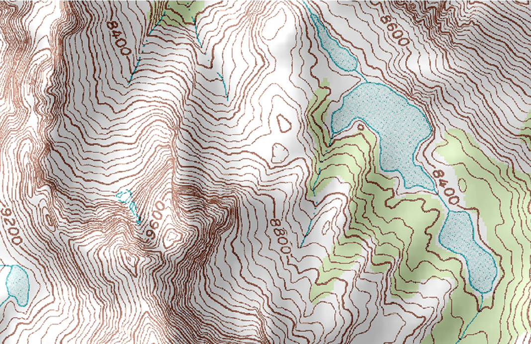
A topography map is another example of a scalar field representation. The map shown below represents the height of the Earth's surface as a function of position. Because the Earth does not shift quickly, we can neglect that this map depends on time. This map mainly displays height by drawing lines along paths of equal height. The land along a single contour is at the same elevation. Neighboring lines are separated by the same difference in height, which gives us information about the steepness of an area. When the density of lines is large (lines are close together), this means that the region is very steep since the height is changing quickly with short distances. This typically represents a peak of a mountain as in the region of about 9600 feet in the map below. Regions of widely separated lines represent flat areas such as valleys as seen near the body of water below. Drawing a line in a scalar field such that every point on the line has the same value in the field is an idea that will be utilized more later.

Figure 11.1.2: Topological Map as a Scalar Field Representation 

Vector Fields

The previous examples were scalar fields because they describe scalar quantities (like temperature or height). Vector fields define a vector, that has both a magnitude and direction, for all positions and times. Vector fields are much more relevant to the topics discussed later in this chapter, so take a while to make sure you can distinguish between the two.

A wind map shown below displays the velocity of the wind at various locations at a fixed time. Because the velocity is a vector, this map must display both the direction and magnitude of wind. The color is used to represent areas of the map where the wind is a fixed magnitude. The arrows show the magnitude and direction of wind at various locations. Like before, although the arrows aren't drawn everywhere on this map, the field defines a magnitude and direction for every point in the map.

 

Figure 11.1.3: Wind Map as a Vector Field Representation 

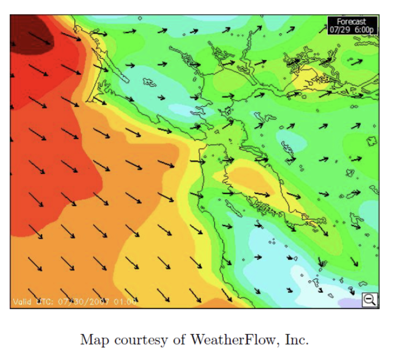
The representation of a vector field presented above, where arrows display the vector field at various locations, is called a field map representation. We will become familiar with other ways to represent vector fields, each of which with its own advantages and disadvantages. The advantage of field maps is that they can be read by eye very quickly, but it omits information about the vector field's scale.

Alert

There may be examples of functions that fit into our definition of "a field" which are probably not very useful. For example, one could define an elephant field in the following way: given a specific position and a specific time, the elephant field describes how many elephants exist there. Certainly this "field" fits into our definition, but it is not a terribly useful thing to consider. We cannot use the "elephant field" to make any new predictions, it is not required by any experiments, and it does not simplify any discussions. It is important to recall that we only consider something a field where it is required by experimental evidence (like the electric and magnetic fields) or it is convenient for discussing the quantity (like temperature).