
11.8: Magnetic Force

( \newcommand{\kernel}{\mathrm{null}\,}\)
Forces on Moving Charged Particles
If we run currents through two parallel wires, something unexpected happens – the wires exert forces on each other! One might be inclined at first to explain this by claiming that putting currents through the wires puts electric charge into them, and that the electric charges are exerting electrical forces on each other. But this is not correct. Current is simply a steady flow of charge – there isn't any charge built-up in the wire. For every electron that enters the wire, a corresponding electron exits it. So the force must have something to do with the motion of the charges. After further experimentation, we find that if we place a stationary net charge near a conducting wire with current, there is no force between them. So apparently there must be motion for both sets of charges in order to exhibit this force. These observations is what eventually led to the connection between electricity and magnetism.
It is far from clear what currents and moving charges have to do with anything related to the fridge magnets or bar magnets that make magnetism familiar to us. The ideas of how a magnetic field affects moving charges were not known until the mid-1800s. Before that, the only thing known about magnetism was that some materials can produce magnetic fields and these attract (or repel) certain kinds of other similar materials, and that the Earth had its own magnetic field which aligns these magnetic materials. These facts were known to the Greeks as early as 600 BC. The question of why certain materials where magnetic while others did not appear to be, and what phenomenon created these magnetic fields was not addressed until 1820.
In 1820, Dutch physicist Hans Christian Ørsted had set up an experiment to show that large electric currents could be used to heat a wire. While demonstrating this to a group of students in his house, he noticed that a compass on his bookshelf changed direction whenever his “kettle” was switched on. After months of investigation, Ørsted concluded that an electric current could create a magnetic field. This was big news at the time, because prior to this only magnetic fields were known to affect other magnetic materials. This was a watershed moment in the history of science, as it was the first link between electric and magnetic phenomena, known as electromagnetism. Originally we experience these as two distinct forces, two distinct fields. Ørsted’s finding was the first step on the road that led humankind to find that these apparently dissimilar phenomena were in fact linked. This unification of seemingly disconnected ideas is still at the core of fundamental research: much hope is placed on possibly unifying all forces in nature.
While this force involves electric charge, it clearly is not electrical in nature. That is, it is altogether different from the Coulomb force. We therefore give it a different name. We call it the magnetic force. Like the electric force, we will explain it in terms of a vector field. And as with the electric force, this will require the two-step theory of first explaining how a charge acts as a source for the field, and then how another charge reacts to being in the presence of a field. We are going to hold off on the first step for now, and focus on the second step, which means we will just start with a magnetic field (without worrying about how it got there beside what we already know about magnets from the previous section), and discuss how the field exerts a force on the moving charge.
We will approach this topic as if we were performing experiments to extract the information we want. Here is a list of our observations from these experiments:
- The strength of the magnetic force on a charge is proportional to the magnetic field through which the charge is moving – This is not surprising, as it was also true for the electric force and field, but more to the point, it really is a result of our definition of magnetic field.
|→FB|∝|→B|
[Note: The traditional variable for magnetic field is B.]
- The strength of the magnetic force on a charge is proportional to the magnitude of the charge – Again, not surprising.
|→FB|∝q|→B|
- The strength of the magnetic force on a charge is proportional to the speed at which the charge is moving though the field – This was mentioned above, and it is the first divergence form the electrical case.
|→FB|∝q|→v||→B|
- The strength of the magnetic force on a charge varies depending upon the relative directions of the magnetic field and the charge's velocity vector – Now this is new! Specifically, we find that the force is zero if the charge happens to be moving parallel to the field, and is its strongest when the field and velocity are perpendicular to each other. Further experimentation reveals that the strength of the force is proportional to the sine of the angle between the field and velocity vectors. Thus, we obtain the magnitude of the magnetic force on a moving charge in an external field:
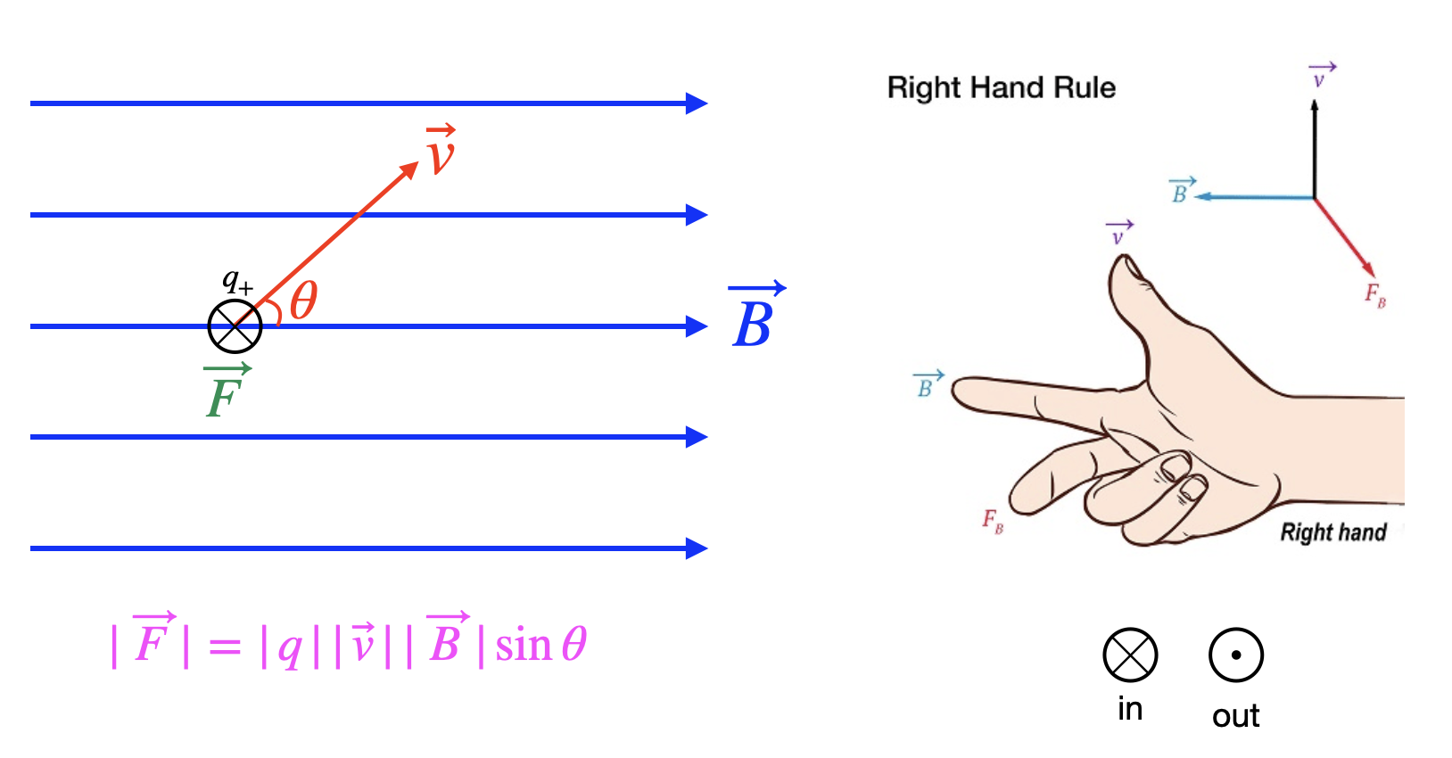
|→FB|=|q||→v||→B|sinθ
- The direction of the magnetic force is perpendicular to both the direction of the velocity and the direction of the magnetic field – This is quite different from the electric case, for which the direction of the force and the field are always in the same or opposite directions.
When combining the magnitude and the direction of the magnetic force, mathematically it is written using the cross product:
→FB=q→v×→B
Since we do not calculate cross-products directly in this course, we can instead determine the magnetic force vector by using using Equation ??? to calculate its magnitude, and using a right-hand-rule for the direction of the magnetic force depicted in the figure below. To use the right-hand (RHR) rule, as the name implies use your right hand, point your thumb in the direction of the charge's velocity, your index finger in the direction of the component of the magnetic field which is perpendicular to the velocity, and your middle figure which is perpendicular to the other two will tell you the direction of the force. It is also important to note that like the case of the electric force, a negatively-charged particle experiences a magnetic force in the opposite direction of a positively-charged particle under the same conditions. Thus, if the charge is negative, you can still apply the same right-hand-rule but flip the result by 180o to obtain the correct direction of the force on a negative charge. The figure below shows the relationship of the velocity, field, and force vectors in an example. It should be noted that the symbols ⊙ and ⊗ will start playing common roles in diagrams from here on, and they represent the directions "out of the page" and "into the page", respectively.
Figure 11.8.1: Magnetic Force Direction and Magnitude
If there is more than one source of magnetic field, we apply the same rules of superposition as we did for electric fields by adding the magnetic field vectors generated by the individual sources to obtain the net field. In addition, there's no reason that electric and magnetic fields can't coexist in the same space. When they do, the force on the point charge is the vector sum of the two forces. The combination (often referred to as the Lorentz force) is therefore:
→F=q(→E+→v×→B)
Before moving on, we should say a word about units. For the equation given above to have proper units, the untis for magnetic field must be force divided by charge-times-velocity. Given how many different names we have for various units, we can of course express this many ways, but once again we will give this quantity its own name:
[B]=[F][q][v]=NC⋅ms=NA⋅m≡T("Tesla")
It turns out that a magnetic field with a magnitude of 1 T is quite strong. It is not beyond common experience (neodymium bar magnets get to this strength), but more commonly encountered magnetic fields (such as that of the Earth, or a compass needle) are significantly less, and it is more common to see these field strengths described in units of Gauss (G), which the simply one ten-thousandth of a Tesla. The strength of the Earth magnetic field near its surface ranges from 0.25 to 0.65 G.
Field From a Moving Point Charge
When we first started discussing magnetism, we noted a force between two current-carrying wires. From there, we focused on the fact that a magnetic field affects only moving electric charges, but it should be equally clear that the source of a magnetic field must also be moving electric charges. One might object that we just said that magnetic fields don't have point sources, so what difference does it make that we insist that the point source be moving? We will see that this makes all the difference, because this leads to a field that doesn't point directly toward or away from that charge – the direction of the field is determined by the direction of the velocity vector.
As different as the magnetic field is from the electric field, there are still so many striking similarities that it is useful to describe the features of the magnetic field from a moving point charge in parallel with the Coulomb electric field. This magnetic analog of the Coulomb field is called the law of Biot & Savart.
- In the Coulomb case, we started with the fact that the field strength is proportional to the magnitude of the charge emitting the field. In the magnetic case, the field strength is also proportional to the magnitude of the charge, but since the charge must also be moving, it turns out that the field strength is also proportional to the charge's speed. This agrees with the observation that there is no magnetic field if the charge is stationary.
- Next we consider how the strength of the field weakens with distance from the source. In this case, the two fields behave identically – with an inverse-square law.
- The direction is where these two fields differ the most. In the Coulomb case, the field points directly toward or away from the point charge. Put another way, if the source charge is at the origin, then the electric field at a position in space described by a position vector →r points in a direction that is parallel to that position vector. The magnetic field, by contrast points perpendicular to that position vector. This doesn't narrow down the direction, however, as there is an entire plane that is perpendicular to this vector. This is where the velocity vector direction comes in – the magnetic field is also perpendicular to the direction defined by the velocity vector. We already know a way of expressing a vector that is perpendicular to two other vectors at the same time – it must be parallel to the cross product of those two vectors.
Field From a Current in a Straight Wire
It is far more common to have physical situations where a magnetic field is created by a current-carrying wire rather than by a moving point charge. We will first study a simple test case: a long straight wire carrying a current. We want to understand the magnetic field produced by this wire, i.e. how strong is its magnitude, where it points (recall it is a vector), and how does it vary with position. In other words, we want to map the magnetic field around the wire.
We will retrace some of Ørsted’s steps. He showed that a current-carrying conductor produces a magnetic field. A simple way to demonstrate this is to place several compass needles in a horizontal plane (for example, the surface of a table) near a long wire placed vertically (running up and down through the table surface). Let’s assume the current direction to be coming from the top and going toward the bottom of the table, as drawn on the left in the figure below. When there is no current in the wire, all needles point in the same direction (magnetic north). As soon as current starts flowing in the wire, all needles will deflect. We have produced a magnetic field!
The first thing that one notices when doing this experiment, is that the needles orient themselves in a recognizable pattern: if we draw a circle on the table with the wire at the center and we place the compasses along the circle, we will notice that all the compass needles will orient themselves tangential to the circle. In other words, the field lines for the magnetic field, →B, generated by long straight wire at a distance r from the wire will have the shape of concentric circles of radius r. For our experiment with the current coming down into the table, we find that the magnetic field direction clockwise along the circles if viewed from the top. The figure below has both the side an the top view (with current going into the page) of the wire. If we flip the direction of the current, the compass needles will still point tangent to the circle, but now their north poles point in a counterclockwise direction.
Figure 11.8.2: Direction of Magnetic Field Around a Current Carrying Wire
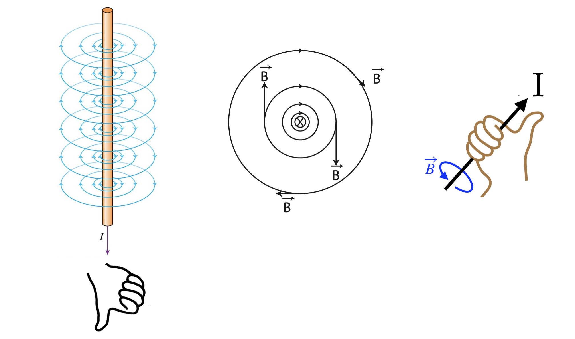
Thus, there is yet another very convenient right-hand-rule for the direction of magnetic field around current carrying wires. It is demonstrated in the figure above. You need to point the thumb of your right hand in the direction of current. Then the curling of your fingers will indicate the direction of the magnetic field circles that are formed around the wire.
Let's mathematically relate every quantity that we have talked about. We expect that all points at the same distance r will have the same magnitude, since the compass needles around a wire arranged in a circle with radius r. It is also not unexpected that the magnitude of the field will be larger if we have a larger current, I. It turns out that the field is proportional to the current. For mathematical reasons we won't go into, when you convert point charges to currents the relationship between magnetic field and distance no longer follows the inverse-square law, but is now proportional to the inverse of distance. Precisely, the magnitude of the magnetic field around a current carrying wire is given by:
|→B|=μoI2πr
The physical constant that makes the units work out for the force is called the permeability of free space:
μo=4π×10−7T⋅mA
Field From a Current in a Circular Wire
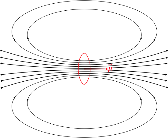
If you have a loop of wire instead, the same principles apply as for a straight wire. The diagram below shows a loop wire with current in the counterclockwise direction as viewed from the right side. Using the RHR for currents, we find the that the field lines go through the loop to the right and circle around counterclockwise on the top and clockwise at the bottom. This generates a dipole magnetic field, and like the electric dipole, the field along its axis points in the direction of the dipole moment. Thus, we see that a loop wire is equivalent to a magnetic dipole, with dipole moment, →μ.
Figure 11.8.3: Magnetic Dipole Field of a Loop
It is possible to stack lots of individual dipoles on top of each other to create a long tube called a solenoid as pictured below. By the law of superposition, the magnetic field inside the solenoid keeps adding with each loop, and as the number of loops increases the field inside becomes approximately constant. It can be calculated that the net field inside the solenoid depends on the current, the length of the solenoid, and the number of turns:
|→B|=μoINL
Figure 11.8.4: Solenoid Magnetic Field
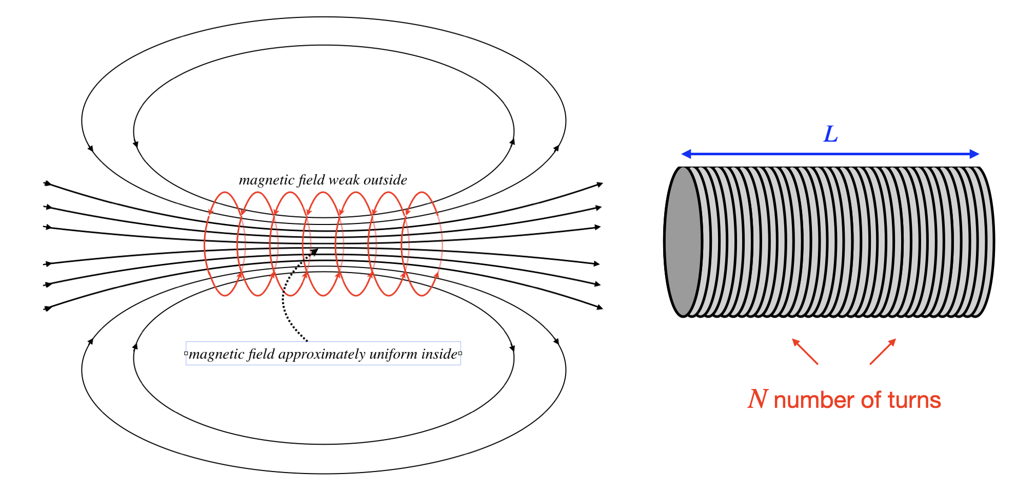
There are a few particularly interesting aspects of the fields of solenoids:
- The field within the solenoid doesn’t change much (it is pretty much uniform).
- The field just outside the solenoid (on its side, not the end) is very weak (basically it is zero).
- The field looks just like that of a bar magnet, but it can be turned on and off by switching the current on or off.
What is a Magnet?
The finding that electricity and magnetism are linked caused a huge revolution in science, but we now want to return to our question of what makes a magnet a magnet. Ørsted showed us that electric currents created a magnetic field, but where are the currents in a magnetized piece of iron? People could not answer this question until the late 1800s, and even then they were met with skepticism. The answer relied on the existence of atoms: in a nutshell, the origins of magnetism are found to be the electric currents produced by the electrons orbiting (i.e. making a current loop) atomic nuclei.
The magnetism of certain materials also depends on spin orientation. Spin endows the electrons with an intrinsic angular momentum. This “intrinsic spin” can only have two possible values (you might have heard that an electron can be “spin up” or “spin down” in your physics or chemistry classes). Spin is a purely quantum mechanical phenomenon, but for the purposes of thinking about magnetism in our current discussion, consider spin an additional way to produce a loop of current (the smallest one you can imagine!)
To summarize, all our experiments point to the following finding: to get a magnetic field, we need a net motion of charge. How does this idea explain magnetism in materials? Imagine helium, an atom with two electrons. Now if these electrons go around in opposite directions, the currents they produce will be opposite to each other. The magnetic field of one current loop will cancel the magnetic field of the other, leading to no net magnetic field. The spin also affects the magnetic field, and if the spins are pointed in the same direction (both up or both down) the field gets stronger, while if they are aligned in opposite directions the field gets weaker. In helium, the spins of the two electrons are paired up-down, so helium would not be very magnetic. As it turns out, helium is an “anti-magnet” and tries to stop any magnetic field going through it. This effect is called diamagnetism and is a manifestation of Lenz's which will be covered in a later section.
However, there are many materials whose atoms have an odd number of electrons but who don't exhibit magnetism, how can that be? So far we have discussed the effects of the magnetic field on individual atoms; we need to consider the possibilities that these atoms are also interacting strongly with each other. Since a material is made up of ∼1023 atoms, tiny effects, like the ones between atoms, can become large if each atom contributes to it. Highly magnetic materials are generally metals, because metals have many outer electrons that act as if they're "free", and can interact strongly with external fields and with each other.
Example 11.8.1
Shown below are four scenarios depicting directions and magnitudes of magnetic field and velocity of charge. The magnitudes of the charges are the same in all cases, but in Scenario 1 and 3 the charge is positive, and in Scenarios 2 and 4 it is negative.
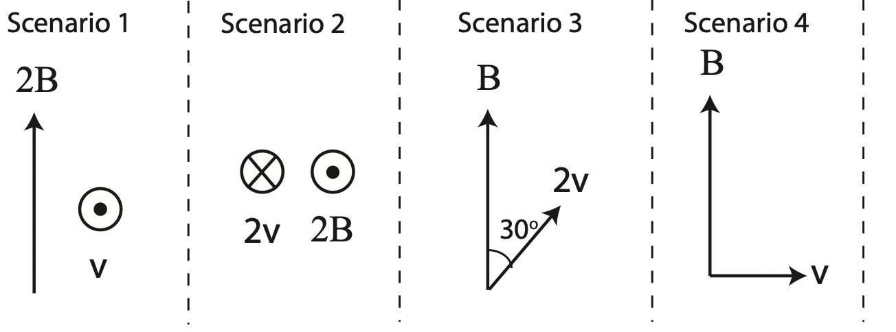
a) Rank the magnitudes, from smallest to largest, of the magnetic force on the charge in each scenario.
b) Find the direction of the force for each scenario.
- Solution
-
a) Scenario 1: F=2vB
Scenario 2: F=0
Scenario 3: F=2vBsin30∘=vB
Scenario 4: F=vB
Ranking: 2<3=4<1
b) Using the force RHR and flipping answer for negative charges:
Scenario 1: left
Scenario 2: force is zero
Scenario 3: out of the page
Scenario 4: into the page
Example 11.8.2
In the figure below a negative charge is moving inside a wire with the current flowing counterclockwise, as shown here. A large magnet is also present with the south pole facing the wire. Find the direction of the magnetic force on the charge.
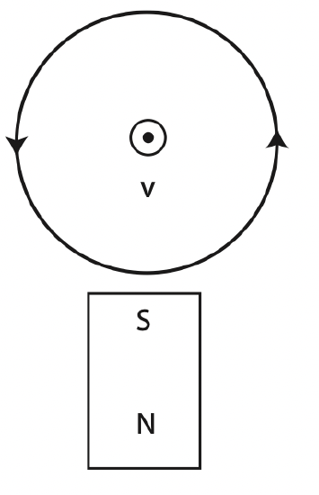
- Solution
-
The RHR for current tells us that the magnetic field due to the wire is point out of the page inside the wire, which is parallel to the motion of the charge, so this field does not contribute to force. Due to the magnet the field points down toward the south pole and away from the north one. Using the RHR for force and flipping answer due to negative charge, we get a magnetic force which points to the left.
Example 11.8.3
Below are two current carrying wires with unknown magnitudes and currents flowing in the opposite directions. Also shown are two electrons and one proton moving in the vicinity of the wires. The arrows represent the direction of motion of each charge. The magnitude and direction of the total magnetic field due to the two wires at the location of the two electrons are equal. The total magnetic field at the location of the proton is out of the page and has a magnitude of μoπ. Each grid square represents a distance of 1m. You may assume that the forces between the charges are negligible.
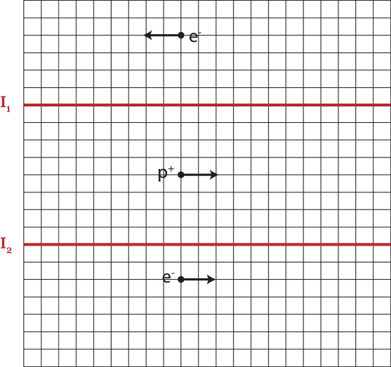
a) Determine the direction of the current in each wire.
b) Calculate the magnitude of the current in each wire.
c) If the current in wire 2 suddenly turned off, determine the direction of force on the electron above the wire 1.
- Solution
-
a) Since the total magnetic field is out of the page at the location of the proton and the currents are in opposite direction, the top wire’s current is to the left and the bottom one is to the right according to the RHR for current.
b) For consistency let’s define out of the page as positive direction and into the page as negative. Thus, the total magnetic field at the location of the proton:
→Btot=→B1+→B2=μo(2π)(4m) (I1+I2)=μoπ
Resulting in:
I1+I2=8A
At the top electron the magnetic field due to wire 1 is into the page and due to wire 2 is out of the page. The magnitude of the total field is:
→Btot=μo2π (I212−I14)
At the bottom electron the magnetic field due to wire 1 is out the page and due to wire 2 is into the page. The magnitude of the total field is:
→Btot=μo2π (I110−I22)
Setting the two equations about equal to each other and solving for I1 in terms of I2:
I1=3521I2
And plugging into the first equation:
3521I2+I2=8A
Resulting in:
I2=3A; I1=5A
c) Based on result in a) the current in wire 1 is to the left, so the magnetic field is into the page above the wire based on the RHR for wires. Using the RHR for force and flipping result for a negative charge the force is up.