8.1: Introduction to Waves

We begin our study of waves in this first unit of Physics 7C with an introduction to waves and then a thorough development of the harmonic plane wave model, which we will use extensively to model and understand a wide variety of wave phenomena.

In this section we will familiarize ourselves with waves by focusing on material waves. These are the disturbances of atoms or molecules in a particular substance. Any sort of ripple that you have seen is a material wave. Some examples include ripples in a pond or a wave on a slinky or a string. Although not visible to the naked eye, sound is modeled by material waves as well.

One of the distinguishing features of physics is that physicists continually strive for general principles and simple models that can be applied to large classes of phenomena. In our study of wave phenomena we consciously take this approach. The focus is on the models and their representations, not on any one of an almost unlimited number of individual examples associated with waves (like sound, light, TV and radio waves, microwaves, etc.) Our goal is to enable you to develop a useful understanding of wave behavior that you can apply to any phenomenon that can be modeled as a wave.

Basic Wave Concepts

There are two important goals associated with the first part of this unit. Firstly, to become familiar with wave phenomena and how we analyze them, and secondly, to sufficiently understand the mathematical representation of one-dimensional harmonic waves. We want to use this mathematical representation as a tool throughout the rest of the course to help us understand the physics of sound, light, and other types of waves.

A material wave is a very common type of internal motion of a material substance. That substance through which the wave propagates is called the medium. In order for material waves to exist there must be forces between neighboring particles in the medium. For simplicity will examine how a disturbance travels and gives rise to wave-like behavior by coloring a medium three different pieces and labeling them as sections 1, 2 and 3 in Figure 8.1.1 below.

Figure 8.1.1: Representation of a Material Wave

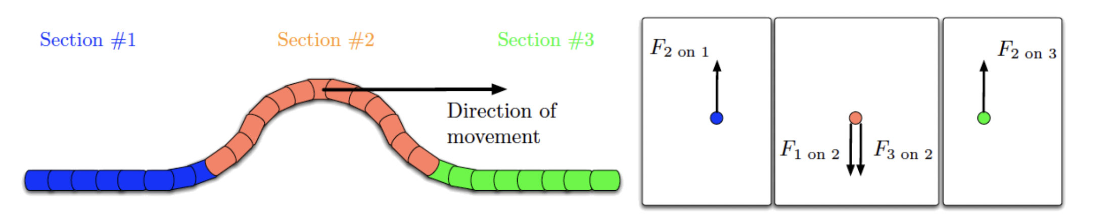
The medium is in equilibrium when it is not being disturbed. If the medium above represents a segment of a rope, then it would lie flat in equilibrium. One can disturb this medium by shaking one end of the rope. In the instant of the wave depicted in Figure 8.1.1, section 2 is displaced from equilibrium as it pulls on sections 1 and 3. The distance from equilibrium is known as the displacement of the medium as the waves passes through it. By Newton's third law, section 2 is pulled down by sections 1 and 3. This is shown by the opposite arrows,\(F_{\text{1 on 2}}=-F_{\text{2 on 1}}\) and \(F_{\text{3 on 2}}=-F_{\text{2 on 3}}\), in the force diagrams above. Thus, section 2 will accelerate downward, back toward equilibrium. This will cause section section 3 to accelerate upward, so a little time later section 3 is displaced like section 2 was. In this way, the disturbance has traveled from section 2 to section 3 without the individual pieces of medium traveling along with it.

Alert

When we describe waves we are describing some kind of motion. We will often speak of the waves moving in space to the right, to the left, or outward from the source. This motion in space, does not refer to the particles which comprise the medium. It is the disturbance or the energy which propagates, defined as the wave. This disturbance occurs due to the interaction between neighboring particles in the medium. These particles oscillate about equilibrium in a wavelike manner, but do not physically travel in space along the wave. In other words, material waves provide a mechanism for transferring energy over considerable distances, without the transport of the medium itself.

You may wonder why the sections exert a force on one another at all. The origin of this force can be traced back to the pairwise interactions you learned about in 7A. Individual atoms have a preferred equilibrium separation distance, and resist being pushed or pulled to maintain that preferred distance. Stretching or compressing the medium causes the atoms to exert forces on their neighbors and to resist forces exerted on them, known as restoring forces. We have simply clumped atoms together into three sections for convenience, but this same discussion applies to individual atoms. The restoring forces responsible for wave behavior are typically strongest in solid materials and negligible in most gaseous materials.

The concepts we introduce when discussing material waves are no different from the concepts that we have already introduced when discussing forces, motion, and atoms. We place such an emphasis on waves as a separate phenomenon because dealing with the form of a wave is often simpler than trying to visualize force diagrams for many different sections of a medium. Eventually we will encounter non-material waves, and this previous exposure to disturbances in material waves will be an invaluable guide.

The disturbance (or, more technically, an oscillation) may be spread throughout the medium and recur continuously at each point (called a periodic wave), or the oscillations may exist for only a limited time at each point (a wave pulse). For example, if you shake one end of a rope depicted in Figure 8.1.1 only one, you will send a wave pulse down the rope. On the other hand, if you continue to shake the rope in a consistent and periodic manner, then you will generate a periodic wave on the rope.

Waves in a medium are started by outside forces that act on some of the particles in the medium to start them oscillating. The object which generates these external forces is known as the source of the wave. External forces are not required to keep a wave going once it has been started. Consider a water wave on the surface of a pond; a rock dropped into the pond is the outside disturbance that starts wave motion. Once started, the ripples expand outward on their own. We don’t have to continue dropping rocks into the pond to keep the ripples moving.

Formal Definition of Waves

It is difficult to come up with a general definition for a "wave". For the moment we will content ourselves by writing down the following definition of a material wave:

A material wave is the large movement of a disturbance in a medium, whereas the particles that make up the medium oscillate about a fixed equilibrium position.

Let’s try again to understand what exactly is moving when describing a wave through an example. Consider ripples expanding in a pond. While there is some movement of the individual water molecules, they merely bob up and down, and they do not travel. It is the ripples that move significantly. The movement of the ripples across the surface of the water is what we mean by a wave. It is not the movement of the individual water molecules, or the disturbance of the surface of water from equilibrium, but rather the movement of the disturbance to different locations in the medium that we call the wave.

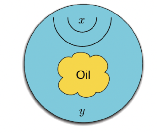
Try an experiment at home to clarify this distinction of motion when describing a wave. Take a bowl of water, and drop a small amount of olive oil on the surface, so that you have a set-up like picture below. If you oscillate your hand gently at the location \(x\), do you get ripples at the location \(y\)? What about the oil? Does it move to the location \(y\)?

Figure 8.1.2: Wave Motion Experiment

Pulse Wave

A pulse is a disturbance with a finite length. For example, if you shook the end of a rope only once you would produce a pulse wave as shown below.

Figure 8.1.3: Wave Pulse 

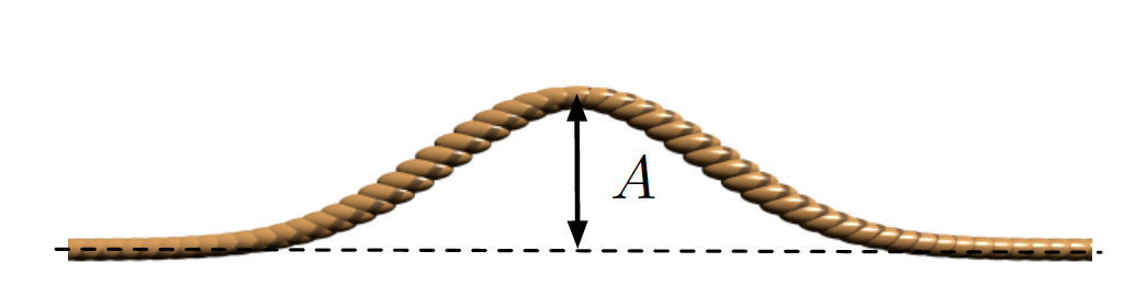
The location of the rope before and after the pulse passes is the equilibrium position. The maximum magnitude of the displacement of the pulse from equilibrium is called the amplitude, \(A\). We define \(A\) to be always positive even if the displacement is below rather than above the equilibrium dashed line shown in the figure above. The amplitude depends on the source, or the amount of energy transferred to the medium by an external object, such as your hand shacking the rope. Another example of a pulse-type wave is the example of a rock thrown into a pond. In this example the rock produces many ripples, but they are a pulse wave because there are a finite amount of ripples with a well-defined beginning and end.

A Periodic Wave

Repeating waves can have many different shapes. One of the simplest to work with looks like a sine or a cosine function. Such waves are called harmonic or sinusoidal waves. They are generated by oscillators moving in simple harmonic motion, like the spring-mass system you studied in 7A. In other words, a harmonic wave can be modeled with motion of each particle in the medium described by spring-mass oscillator. If you hold one end of a rope and jiggle it up and down in simple harmonic motion, moving your hand in a periodic repeating manner, you will generate harmonic waves. If you were to take a picture of the wave, it might look like the figure below.

Figure 8.1.4: Periodic Wave 

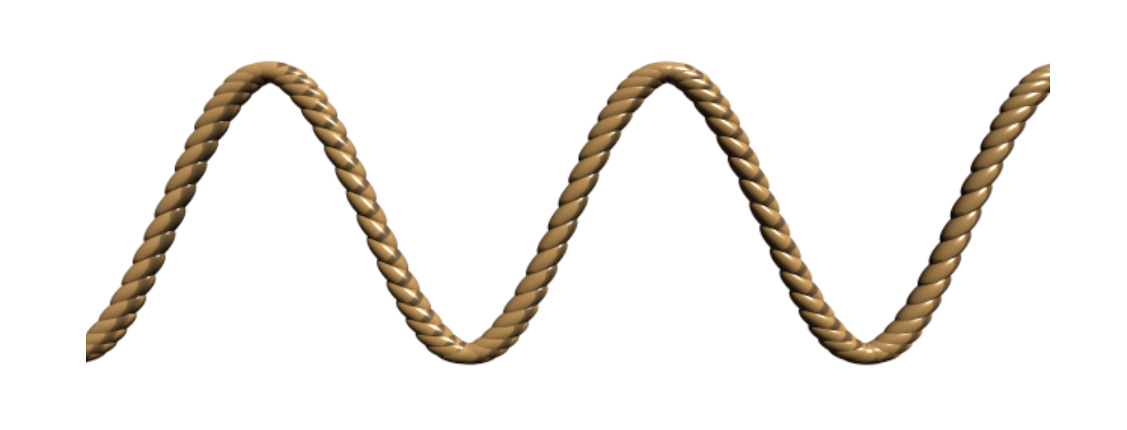
When you "take a picture" of a wave you capture its shape at some instance of time, which we call the snapshot of the wave. This can be represented graphically as shown below. Here \(x\) is the distance along the rope, and the displacement, \(y\), represents how far the rope is displaced from equilibrium. 

Figure 8.1.5: Graphical Representation of a Harmonic Wave at a Fixed Time ("Snapshot")

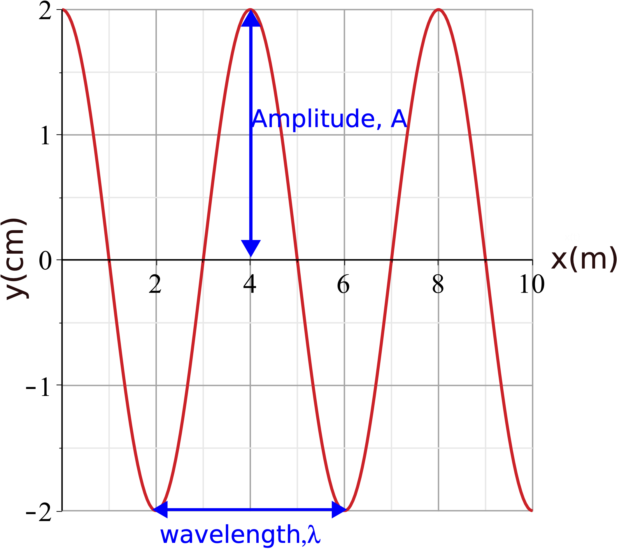
Like the wave pulse, a repeating wave has a well-defined equilibrium position and an amplitude, \(A\). In Figure 8.1.5 the equilibrium position is at y=0 cm, and the amplitude is 2 cm. Compared to a wave pulse, a repeating wave has two new parameters. The first is the wavelength, \(\lambda\), which tells us the shortest distance (along the direction of wave motion) between identical parts of the wave. In other words, the wavelength represents the length of the spatial cycle of the wave as marked in Figure 8.1.5 above. In this figure \(\lambda= 4\) m. 

The second new parameter is the period ,\(T\) , the time it takes for the wave to look exactly the same. In other words, the wavelength tells us how the wave repeats in space, while the period tells us how the wave repeats in time. One period is the time it takes for the wave to move a distance of one wavelength, since it will look the same after one cycle. Oscillators in the medium go through one cycle during the time of one period, such as a spring-mass returning to its starting position. Pulse-type waves, which do not repeat, do not have periods or wavelengths. The wave period is determined by how often the source is disturbing the medium. If you were generating a harmonic wave on a rope, you can determine the period by measuring how long it takes for your hand to move up and back down.

Since the graph in Figure 8.1.5 shows the wave for a fixed time, so it gives us no information about the period which is time-dependent. To give a representation of the temporal characteristic of the wave, we need a new graph. Since there are two variables which describe the wave, space and time, in order to graph the wave changing with time we now need to represent it at a fixed position. If we were to paint a red dot on the rope at some fixed \(x\) value, and then plot the position of only that dot against time, we would find how that particular point moves in simple harmonic motion (see Figure 8.1.7 below). Thus, when representing the motion of the wave as a function of time, we are showing the harmonic oscillation of one specific particle in the medium which is at some fixed location in space. It takes the same amount of time for the "dot" to return to an initial position as it does for the whole wave to return to an initial configuration, as you can see in Figure 8.1.7. An example of a displacement versus time graph is shown below.

Figure 8.1.6: Graphical Representation of a Harmonic Wave at a Fixed Position

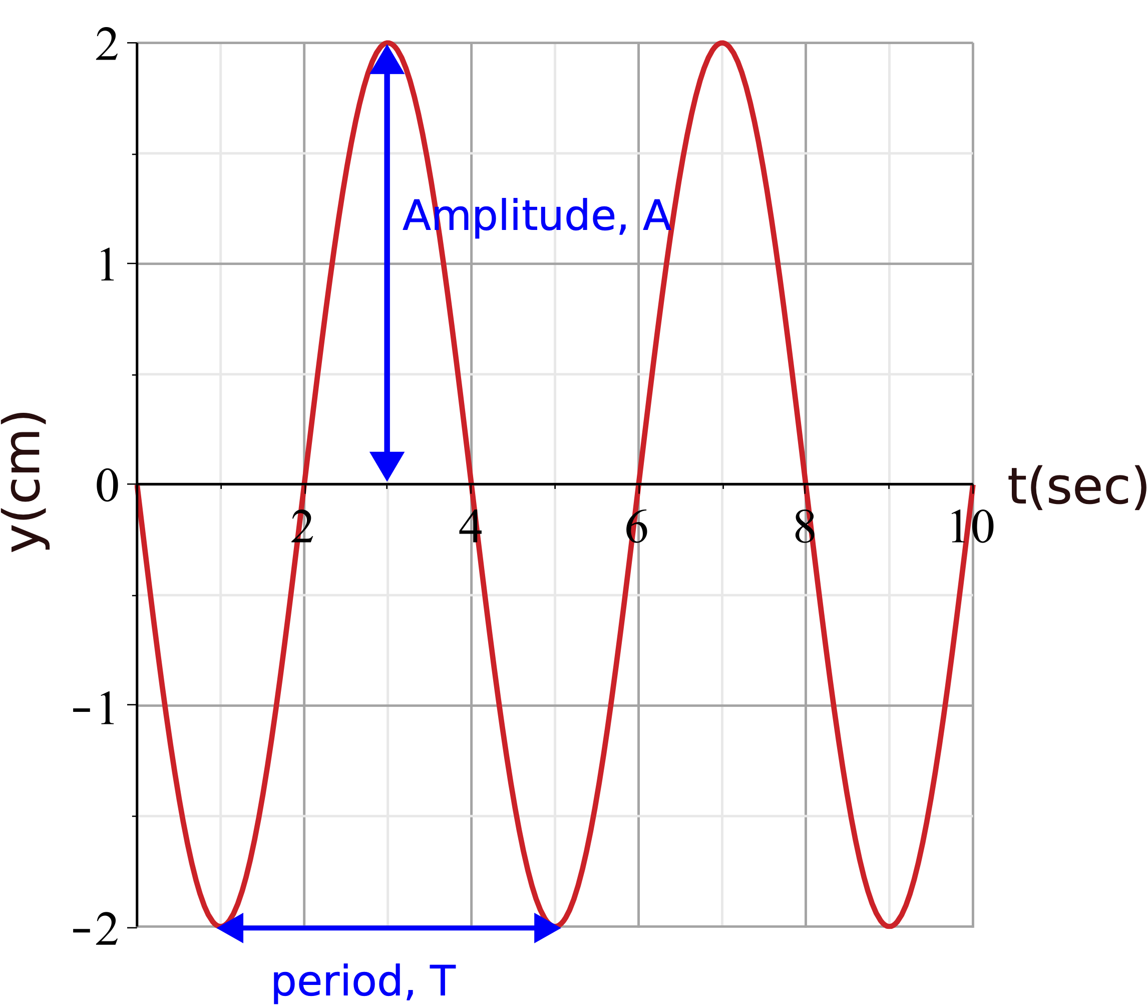
The period representing one temporal cycle is 4 seconds in the graph above. Assuming that figures 8.1.5 and 8.1.6 represent the same wave, the information they provide must be consistent. For example, both graphs show the same amplitude of 2 cm. The maximum displacement, known as the crest of the wave, is at 2 cm, the minimum displacement, the trough of the wave, is at -2 cm, and the midpoint between the crest and the trough is the equilibrium position, here at y=0 cm. In Figure 8.1.5 we see that the particle at position x=0 m is at a crest, position x=1 m is at equilibrium, and x=2 m is at a trough. Let us assume that Figure 8.1.5 is a snapshot at t=0 sec. Since Figure 8.1.6 shows t=0 sec at equilibrium, that means that the position it represents has to be at equilibrium in Figure 8.1.5. Thus, possible positions for the time-dependent plot in Figure 8.1.6 could be x=1, 3, 5, etc, where the displacement is at equilibrium in Figure 8.1.5.

The period is the amount of time for one cycle. Another useful measure of the periodicity of a wave is the number of cycles that fit in some unit of time, known as the frequency. Frequency is the reciprocal of the period:

\[T = \dfrac{1}{f}\label{Tf}\]

Typically, period is measured in seconds and frequency is measured in units called Hertz, Hz (1 Hz = 1 s^-1). The period is the time between the arrival of adjacent crests of the wave, while the frequency is the number of crests that pass by per second. This means the red dot in Figure 8.1.7 completes an \(f\) number of up-and-down cycles every second. Equivalently, if you focus on a specific position in space, wave will return to the same configuration an \(f\) number of times every second.

Dimensionality

The examples seen above are called one-dimensional waves because the wave only travels in one direction. We arbitrarily called that direction the \(x\)-axis. If a wave spreads out on a surface instead, then it is a two-dimensional wave. For example, ripples on the surface of a pond represent a two-dimensional water wave. A wave that spreads outward in all directions is a three-dimensional wave. Examples of three-dimensional waves are typical sound and light waves.

An important distinction between these waves is that the amplitude \(A\) of the waves is only constant for one-dimensional waves. Two-dimensional and three-dimensional waves have amplitudes that depend on the distance from the source of the disturbance. Ripples in a pond become smaller as they spread out, and the brightness (amplitude of light) and loudness (amplitude of sound) of light and sound waves, respectively, decreases with distance away from the sources. This is a consequence of conservation of energy, as a wave propagates outward in multiple dimensions, the energy it carries must be spread over a region of increasing size.

Polarization

Material waves and electromagnetic waves have a characteristic called polarization. The polarization relates the direction of wave displacement to the direction of wave motion. For material waves, we are going to define two types of polarization:

• Transverse Polarization: A material wave is transverse if the displacement from equilibrium is perpendicular to the direction the wave is traveling. Below is a transverse wave since the wave is traveling to the right, while the oscillations in the medium are vertical, or perpendicular to the motion. The "red dot" represents one oscillator moving up and down periodically as the wave propagates to the right through the medium. An example of a transverse wave, is a wave generated on a rope or string as in Figure 8.1.4. A surface water wave is another example, since the oscillations of the water particles are in the vertical direction while the wave propagates on the two-dimensional plane of the water surface.

Figure 8.1.7: Transverse Wave

• Longitudinal Polarization: A material wave is longitudinal if the medium displacement from equilibrium is in the same direction that the wave is traveling. In most examples of longitudinal waves that we explore, this displacement occurs as periodic compressions (region of more dense medium) and rarefactions (regions of less dense medium) of the material. The figure below shows an example of a longitudinal wave on a spring (or slinky). The most common example of longitudinal waves are sound waves, which we will discuss in more detail in a later section.

Figure 8.1.7: Longitudinal Wave

Although, transverse waves resemble physically the plots that we drew in figures 8.1.5 and 8.1.6, we represent harmonic longitudinal wave exactly the same way using sinusoidal functions. The displacement on the y-axis in figures 8.1.5 and 8.1.6 does not need to represent the physical depiction of the wave, but rather it shows the distance from equilibrium in the medium. As in the transverse wave, the red dot in the longitudinal waves oscillates sinusoidally. Locations of compressions represent crests while rarefaction represent troughs.

Wave Speed

The wave speed, \(v_{\text{wave}}\), is the speed at which the disturbance propagates through the medium. One way of thinking about the wave speed is that it is the speed someone who was riding the wave on a surfboard would travel. It is not the speed of the oscillations of the individual particles making up the medium. In fact, from 7A we know that the speed of a harmonic oscillator (spring-mass) is not a constant, but changes with distance from equilibrium. The speed is maximum at equilibrium, and decreases as the oscillator gets further away from equilibrium, reaching zero at the maximum distance from equilibrium. 

To a good approximation \(v_{\text{wave}}\) depends only on properties of the medium, not on wave amplitude or frequency. For large waves, or for waves with extreme frequencies, this approximation breaks down. For now, we simplify our discussion by ignoring dependence of wave speed on amplitude (we do not work with big wave in 7C). We will also ignore dependence of speed on frequency, until we discuss refraction of light waves in a later chapter.

The definition of speed from 7B can be written as:

\[\textrm{speed} = \dfrac{\textrm{distance travelled}}{\textrm{time spent}}\]

One period is the shortest amount of time before the wave looks exactly the same. When the wave looks exactly the same again, it has moved a distance of one wavelength by definition. Since it take the wave a time of one period to travel a distance of one wavelength, the wave speed can be written as:

\[v_{\text{wave}} = \dfrac{\lambda}{T}=\lambda f\]

The second equality above uses the definition of frequency from Equation \ref{Tf}. As an example of how the medium determines the wave speed we can look at a material wave on a stretched (characterized by tension) medium, such as a rope or a rubber hose. Both transverse waves and longitudinal waves are possible on a stretched strings or ropes. The speed, \(v_{\text{wave}}\), of transverse waves on a stretched string depends on the properties of the string that affect its elasticity and its internal properties. For a string that is thin compared to its length, the relation between the wave speed to the string properties is given by:

\[v_{\text{wave}} = \sqrt{\dfrac{T}{\mu}}\]

where \(T\) is the tension in the string and \(\mu\) is its mass density, mass per unit length (\(\mu=m/L)\). We can make some sense of the formula by considering the diagram in Figure 8.1.1. The tension is (roughly) the force that one piece of string exerts on another. The tighter the string the higher the tension. As we learned, a material wave is a disturbance that propagates by one piece of the medium exerting a force on its neighbors, it is logical that an increase in tension results in an increase in the wave speed. Stronger forces will lead to greater acceleration. When the string is particularly heavy, the forces between pieces of the string result in less acceleration, so it also intuitive that as \(\mu\) increases the wave speed decreases. The ability to control the wave speed is critical for stringed instruments like a guitar or a violin, which is why they have tuning knobs at one end (to control the tension), and the strings are of different mass (for different values of \(\mu\)). We will discuss string instruments in more detail when we cover standing waves in later sections.