8.6: Beats

So far we have focused on interference between two waves with the same frequency, and thus, wavelength. Interesting phenomena emerges when two waves with different frequencies interfere. To analyze this, let us start with a simplified one-dimensional situation of observing interference to the right of two speakers. In this case, the wavelengths of the two waves are different, since their frequencies are different as depicted in the figure below.

Figure 8.6.1: Wave Interference with Different Frequencies

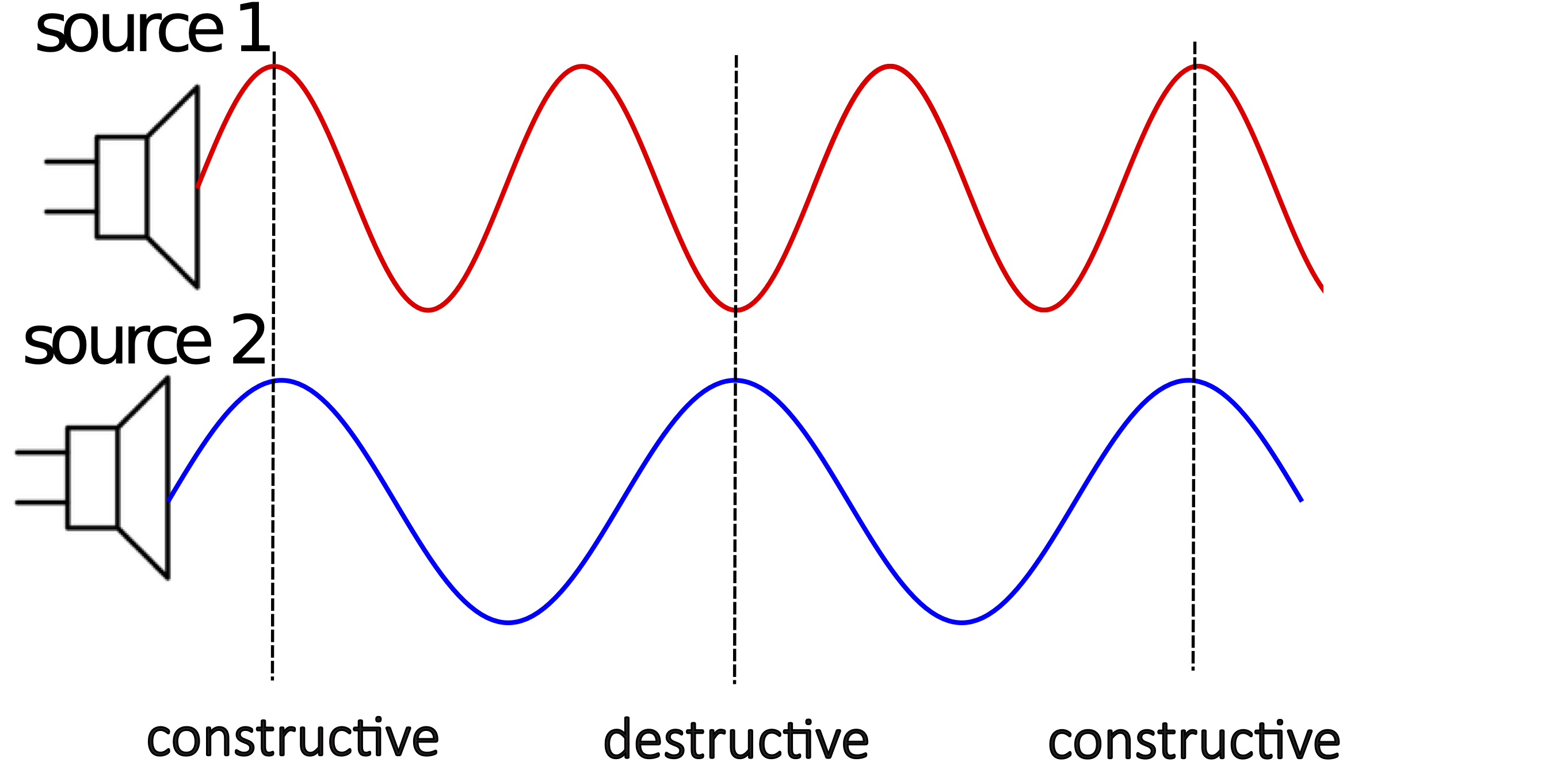
The figure above shows that interference is no longer fixed to the right of the speakers. In the previous section we determined that in this one-dimensional situation the type of interference is fixed for a given position, for which one can determine the difference in phase constants and path length between the two speakers. In other words, for a specific speaker set-up an observer on the right of the speaker always heard either maximum loudness, silence, or something in between. In this case, however, there are locations of destructive, constructive, and partial interference to the right of the speakers. The diagram above is a snapshot of the two waves at some particular time. If you are standing at the most right constructive interference location marked in the figure, you hear a sound of maximum intensity. However, at the later time, since the waves are traveling to the right, the location in the middle where interference is destructive will reach the location of the constructive interference on the right, so the observer will hear no sound. And some time even later, the most left location of constructive interference will reach the observer's location, so they will hear a loud sound again.

Unlike for the case of equal frequencies, we conclude that an observer at a fixed location now hears the intensity of sound changing periodically. In other words, the combined amplitude leading to a specific type of interference is now time-dependent. We call this phenomena beats, since the sound is now literally beating from loud to silent and back to loud, like a drum being hit in a periodic manner. This phenomena is especially relevant for two frequencies which are very closer together, since only then the beats can be perceived by humans. When the difference between the frequencies is large, the beats become too frequent for our ears to distinguish them.

Since we are combining two wave equations with different frequencies resulting in a time-dependent amplitude, the combined wave can no longer be described by a simple sinusoidal wave equation. However, it is still periodic since the amplitude change is periodic. The figure below shows an example of a combined wave from two sinusoidal waves with two different frequencies. The two top plots represent the two individual waves, while the bottom one is the combined one.

Figure 8.6.2: Beats

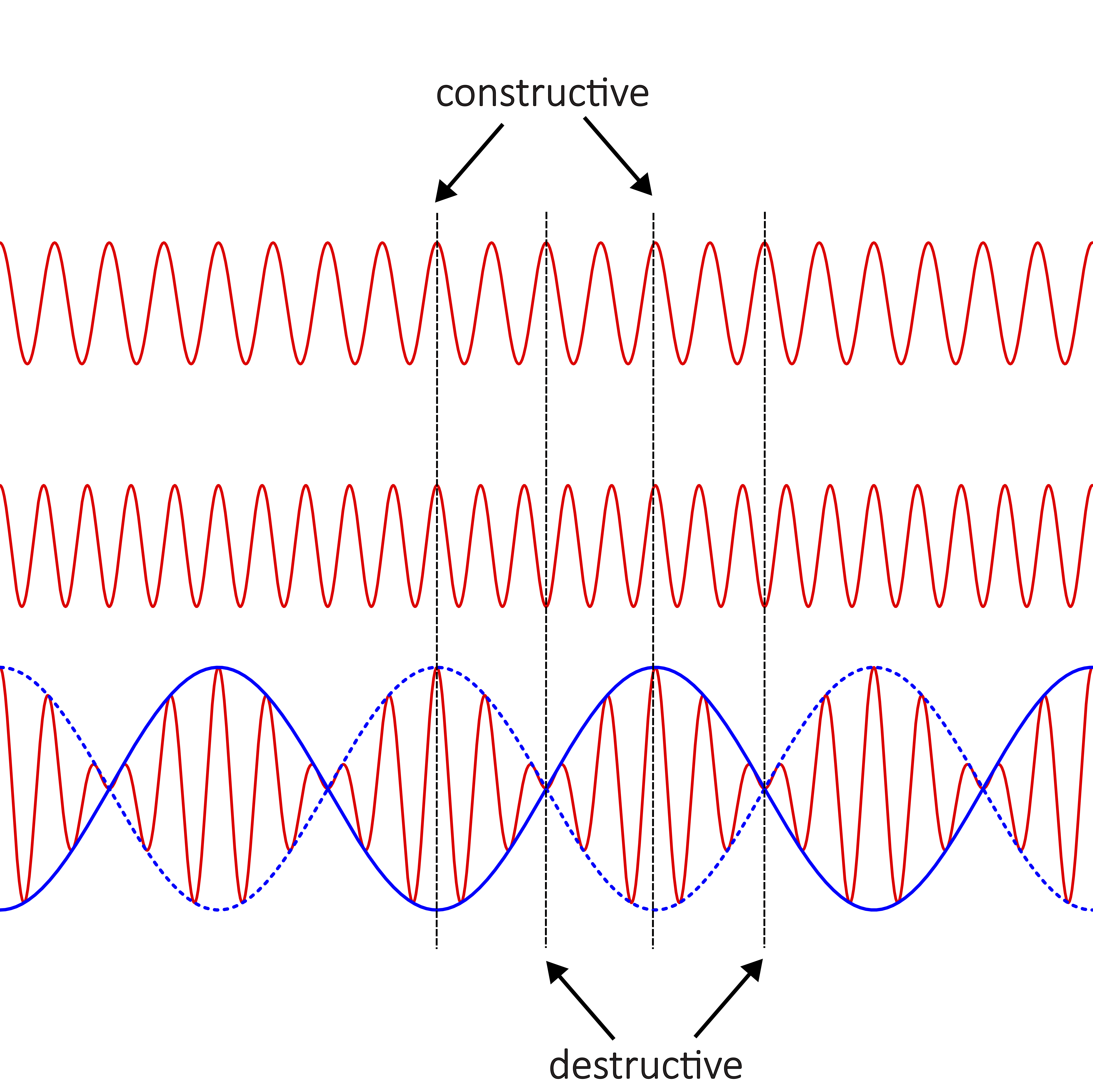
The blue envelope wave on the combined plot outlines the change in amplitude. One can see when the envelope function is at peak, the two individual wave overlap at the same displacement (crests in this figure) resulting in constructive interference at that location. When the envelope function is at equilibrium, the displacements of the individual waves are cancelling (one is at a crest while the other one is at a trough) resulting in destructive interference. This is a snapshot of the combined wave at a fixed time. If you are standing at a fixed position, this wave will move in time, so you will be hearing a periodic intensity of constructive and destructive interference. The period of this time-dependent interference, or beats, is half the period of the envelope function drawn above. The intensity of the sound is the square of the amplitude, so constructive interference (maximum intensity) occur every time the envelope wave is at a crest or a trough, or every half a cycle of the envelope function. Likewise, the envelope function has two locations of zero amplitude for every cycle. The frequency with which beats are heard is known as the beat frequency. For example, a beat frequency of 1 Hz means that the observer is hearing a beat (a loud sound) one time every second.

We can also determine the beat frequency mathematically in terms of the original frequencies of the two waves. The total phase difference between two waves with different frequencies and wavelengths can be written as:

\[\Delta\Phi=2\pi t\Delta\left(\dfrac{1}{T}\right)+2\pi \Delta\left(\dfrac{x}{\lambda}\right)+\Delta\phi_o\label{Phi-tot}\]

To determine the beat frequency, we want to find the time it takes for the interference pattern to repeat itself. Let us assume that at some specific time an observer standing at a fixed location hears constructive interference (the loudest sound from the combined waves). Let us define this time as \(t=0\) sec. Therefore, Equation \ref{Phi-tot} becomes:

\[\Delta\Phi=2\pi \Delta\left(\dfrac{x}{\lambda}\right)+\Delta\phi_o=0\]

At time later time which we define as the beat period, \(T_b\), the observer will again hear constructive interference. This implies that the phase difference increased from 0 to \(2\pi\). The path length difference and the phase constant difference is not time-dependent as long as the observer stays put, so the sum of the second two terms in Equation \ref{Phi-tot} remain zero at \(t=T_b\). Therefore, the total phase difference at \(t=T_b\) is:

\[\Delta\Phi=2\pi T_b\Delta\left(\dfrac{1}{T}\right)=2\pi T_b\left(\dfrac{1}{T_1}-\dfrac{1}{T_2}\right)=2\pi\]

Re-writing the above equation in terms of frequency and solving for the beat frequency, we get:

\[2\pi\dfrac{f_1-f_2}{f_b}=2\pi\Longrightarrow f_b=|f_1-f_2|\label{fbeat}\]

The absolute value in the equation above implies that the beat frequency which is the difference between two frequencies is a positive value, since frequency cannot be negative. Thus, the absolute value assure that the the beat frequency is positive, if you happen to subtract the larger frequency from the smaller one. You can see from this results that the difference in the two frequencies needs to be small for beats to have a meaningful interpretation to the human ear. It is very difficult to distinguish even 10 individual beats in a short time span of one second.

Another important property of beats is the carrier frequency. This frequency is approximately the frequency of the "small" oscillations within the envelop function. In other words, in combined plot of Figure 8.6.2, the carrier period would be the time between two consecutive peaks (approximately). The carrier frequency, \(f_c\), is the pitch you hear coming from the sound which is beating, and it turns out to be simply the average of the two original frequencies:

\[f_c=\dfrac{f_1+f_2}{2}\]

Digression: Beat Wave Equation

We can mathematically determine that beat and carrier frequencies by adding two wave functions of waves with different frequencies. Recall, for sound waves we represent the displacement in terms of pressure, with equilibrium displacement at atmospheric pressure, which we set here to zero for simplicity. The two wave function can be written as:

\[P_1(x,t)=P_o\sin\left(\dfrac{2\pi}{T_1}t-\dfrac{2\pi}{\lambda_1}x+\phi_1\right),~~~P_2(x,t)=P_o\sin\left(\dfrac{2\pi}{T_2}t-\dfrac{2\pi}{\lambda_2}x+\phi_2\right)\nonumber\]

Let us assume that at some location and instance of time which we define as x=0 m and t=0 sec the interference is constructive, such that there is no relative phase constant difference between the two waves, \(\phi_1=\phi_2=0\). We want to see how the wave changes as a function of time at any position, so we choose x=0 m for convenience. Also, we will express the wave functions in terms of frequency instead of period. Thus, the sum of the two wave functions simplifies to:

\[P_{tot}(t)=P_o\sin(2\pi f_1t)+P_o\sin(2\pi f_2t)\nonumber\]

Here we need to use a trigonometric identity: 

\[\sin\alpha+\sin\beta=2\cos\dfrac{\alpha-\beta}{2}\sin\dfrac{\alpha+\beta}{2}\nonumber\]

Applying this identify, we then get:

\[P_{tot}(t)=2P_o\cos\left(2\pi\dfrac{f_1-f_2}{2}t\right)\sin\left(2\pi\dfrac{f_1+f_2}{2}t\right)\nonumber\]

The above function is not the simple wave function with one sine term that we are familiar with, but represents the combination of the two waves. We can think of the second sine function as representing the carrier wave with the carrier frequency of \(f_c=(f_1+f_2)/2\). The quantity \(2P_o\) multiplied by the cosine function represents the time-dependent amplitude of the combined wave. From the equation, we can be that frequency of this amplitude is \((f_1-f_2)/2\). The beat frequency is twice this value, since for each cycle of the envelope function there are two beats, one crest and one trough both representing maximum intensity. This results in the same expression for beat frequency we obtain in Equation \ref{fbeat}, \(f_b=f_1-f_2\). The maximum amplitude is \(2P_o\) which exactly corresponds to constructive interference when the amplitudes of the two original waves are added.

Musicians use the principles of beats to tune their instruments. Frequencies on strings which are confined between two ends, like a guitar string, are determined mainly by the length and the speed of the wave on the string, as we will see in a later section on standing waves. The source no longer has control of the frequencies that it generates on the string, precisely because the ends of the string are confined. This is very different from what we have learned so far, so stay tuned! When tuning a string instrument, the musician changes the tension of the string, which in turn changes the speed and results in a different frequency. They find the desired frequency by using tuning forks (at least this was the main method before tuning apps). A tuning fork has a predetermined frequency based on its physical properties at which it generates a sound when someone strikes it. Thus, with multiple turning forks of different frequencies a musician can tune all the strings to their desired frequencies. They do this by hitting the tuning fork and plucking or striking the string of the instrument at the same time. If the musician hears a beat, the string is out of tune. Then, they will adjust the tension until beats are no longer heard, implying that the string is vibrating at the exact same frequency as the tuning fork. Since the string which is out-of-tune is typically very close to the desired frequency, this results in a small beat frequency which can be easily heard by a human ear.

Example \(\PageIndex{1}\)

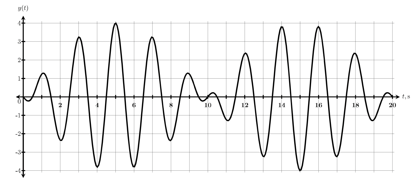
The graph below shows a combination of two waves interacting at a particular point in space. Determine the frequencies of each wave.

Solution

The plot above is the sum of the two waves with different frequencies. The carrier frequency can be found from the period of the small oscillations inside the beat envelope. From the plot we see that the distance in time between any two consecutive peaks is 2 seconds, resulting in a carrier frequency:

\[f_c=\dfrac{1}{T_c}=\dfrac{1}{2s}=0.5Hz=\dfrac{f_1+f_2}{2}\nonumber\]

The beat period can also be obtained from by measuring the time that passed between locations of biggest amplitude. This location does not have to be a crest, but can also be a trough, since the intensity of a wave is proportional to the square of amplitude. In this plot, we see the largest amplitude at t=5 sec. The next time that we observe the same amplitude is at t=15 sec. Therefore, the beat period is 10 sec, and the beat frequency is expressed as:

\[f_b=\dfrac{1}{T_b}=\dfrac{1}{10s}=0.1Hz=f_1-f_2\nonumber\]

where we have assume that the bigger frequency is \(f_1\). Now we can solve for the individual values of frequency, \(f_1\) and \(f_2\), since we have two equations and two unknowns. Plugging in beat frequency into the carrier frequency equation we get:

\[f_c=0.5Hz=\dfrac{f_1+f_2}{2}=\dfrac{f_1+f_1-0.1}{2}=f_1-0.05\Longrightarrow f_1=0.5+0.05=0.55 Hz\nonumber\]

Solving for the other frequency using the beat frequency equation:

\[f_2=f_1-0.1=0.55-0.1=0.45 Hz\nonumber\]

Example \(\PageIndex{2}\)

Three dolphins, Fin, Jumpy, and Clicker are communicating in water by emitting sounds of various frequencies. Fin and Clicker are both stationary. They are emitting a sound of the same frequency of 5000 Hz, while Jumpy is not emitting a sound. As Jumpy moves toward Clicker and away from Fin, he hears a beat frequency of 40 Hz. The speed of sound in water is 1500 m/s. Calculate Jumpy’s speed.

 

Solution

If Jumpy was stationary, he would hear the same frequency coming from both Clicker and Fin, and therefore, would not hear any beats. But since Jumpy is moving toward and away from a sound source, his perceived frequencies of both sources are Doppler shifted, resulting in beats. The observed frequency by Jumpy of Clicker’s sound, \(f_{oC}\), is due to the observer moving, Jumpy moving at speed \(v_J\), toward a stationary source with frequency emitted by source Clicker, \(f_C\):

\[f_{oC}=\dfrac{v+v_J}{v}f_C\nonumber\]

The observed frequency by Jumpy of Fin’s sound, \(f_{oF}\), is due to the observer moving away from the stationary source with frequency emitted by source Fin, \(f_F\):

\[f_{oF}=\dfrac{v-v_J}{v}f_F\nonumber\]

Setting the source frequencies equal to each other, \(f_C=f_F\equiv f_s\), and subtracting the two equations to determine the beat frequency we get:

\[f_b=f_{oC}-f_{oF}=\dfrac{v+v_J-v+v_J}{v}f_s=\dfrac{2v_Jf_s}{v}\nonumber\]

Solving for Jumpy's speed:

\[v_J=\dfrac{f_b v}{2f_s}=\dfrac{40Hz\times 1500 m/s}{2\times 5000Hz}= 6\dfrac{m}{s}\nonumber\]