9.6: Quantum Harmonic Oscillator
- Page ID
- 77396
\( \newcommand{\vecs}[1]{\overset { \scriptstyle \rightharpoonup} {\mathbf{#1}} } \)
\( \newcommand{\vecd}[1]{\overset{-\!-\!\rightharpoonup}{\vphantom{a}\smash {#1}}} \)
\( \newcommand{\id}{\mathrm{id}}\) \( \newcommand{\Span}{\mathrm{span}}\)
( \newcommand{\kernel}{\mathrm{null}\,}\) \( \newcommand{\range}{\mathrm{range}\,}\)
\( \newcommand{\RealPart}{\mathrm{Re}}\) \( \newcommand{\ImaginaryPart}{\mathrm{Im}}\)
\( \newcommand{\Argument}{\mathrm{Arg}}\) \( \newcommand{\norm}[1]{\| #1 \|}\)
\( \newcommand{\inner}[2]{\langle #1, #2 \rangle}\)
\( \newcommand{\Span}{\mathrm{span}}\)
\( \newcommand{\id}{\mathrm{id}}\)
\( \newcommand{\Span}{\mathrm{span}}\)
\( \newcommand{\kernel}{\mathrm{null}\,}\)
\( \newcommand{\range}{\mathrm{range}\,}\)
\( \newcommand{\RealPart}{\mathrm{Re}}\)
\( \newcommand{\ImaginaryPart}{\mathrm{Im}}\)
\( \newcommand{\Argument}{\mathrm{Arg}}\)
\( \newcommand{\norm}[1]{\| #1 \|}\)
\( \newcommand{\inner}[2]{\langle #1, #2 \rangle}\)
\( \newcommand{\Span}{\mathrm{span}}\) \( \newcommand{\AA}{\unicode[.8,0]{x212B}}\)
\( \newcommand{\vectorA}[1]{\vec{#1}} % arrow\)
\( \newcommand{\vectorAt}[1]{\vec{\text{#1}}} % arrow\)
\( \newcommand{\vectorB}[1]{\overset { \scriptstyle \rightharpoonup} {\mathbf{#1}} } \)
\( \newcommand{\vectorC}[1]{\textbf{#1}} \)
\( \newcommand{\vectorD}[1]{\overrightarrow{#1}} \)
\( \newcommand{\vectorDt}[1]{\overrightarrow{\text{#1}}} \)
\( \newcommand{\vectE}[1]{\overset{-\!-\!\rightharpoonup}{\vphantom{a}\smash{\mathbf {#1}}}} \)
\( \newcommand{\vecs}[1]{\overset { \scriptstyle \rightharpoonup} {\mathbf{#1}} } \)
\( \newcommand{\vecd}[1]{\overset{-\!-\!\rightharpoonup}{\vphantom{a}\smash {#1}}} \)
\(\newcommand{\avec}{\mathbf a}\) \(\newcommand{\bvec}{\mathbf b}\) \(\newcommand{\cvec}{\mathbf c}\) \(\newcommand{\dvec}{\mathbf d}\) \(\newcommand{\dtil}{\widetilde{\mathbf d}}\) \(\newcommand{\evec}{\mathbf e}\) \(\newcommand{\fvec}{\mathbf f}\) \(\newcommand{\nvec}{\mathbf n}\) \(\newcommand{\pvec}{\mathbf p}\) \(\newcommand{\qvec}{\mathbf q}\) \(\newcommand{\svec}{\mathbf s}\) \(\newcommand{\tvec}{\mathbf t}\) \(\newcommand{\uvec}{\mathbf u}\) \(\newcommand{\vvec}{\mathbf v}\) \(\newcommand{\wvec}{\mathbf w}\) \(\newcommand{\xvec}{\mathbf x}\) \(\newcommand{\yvec}{\mathbf y}\) \(\newcommand{\zvec}{\mathbf z}\) \(\newcommand{\rvec}{\mathbf r}\) \(\newcommand{\mvec}{\mathbf m}\) \(\newcommand{\zerovec}{\mathbf 0}\) \(\newcommand{\onevec}{\mathbf 1}\) \(\newcommand{\real}{\mathbb R}\) \(\newcommand{\twovec}[2]{\left[\begin{array}{r}#1 \\ #2 \end{array}\right]}\) \(\newcommand{\ctwovec}[2]{\left[\begin{array}{c}#1 \\ #2 \end{array}\right]}\) \(\newcommand{\threevec}[3]{\left[\begin{array}{r}#1 \\ #2 \\ #3 \end{array}\right]}\) \(\newcommand{\cthreevec}[3]{\left[\begin{array}{c}#1 \\ #2 \\ #3 \end{array}\right]}\) \(\newcommand{\fourvec}[4]{\left[\begin{array}{r}#1 \\ #2 \\ #3 \\ #4 \end{array}\right]}\) \(\newcommand{\cfourvec}[4]{\left[\begin{array}{c}#1 \\ #2 \\ #3 \\ #4 \end{array}\right]}\) \(\newcommand{\fivevec}[5]{\left[\begin{array}{r}#1 \\ #2 \\ #3 \\ #4 \\ #5 \\ \end{array}\right]}\) \(\newcommand{\cfivevec}[5]{\left[\begin{array}{c}#1 \\ #2 \\ #3 \\ #4 \\ #5 \\ \end{array}\right]}\) \(\newcommand{\mattwo}[4]{\left[\begin{array}{rr}#1 \amp #2 \\ #3 \amp #4 \\ \end{array}\right]}\) \(\newcommand{\laspan}[1]{\text{Span}\{#1\}}\) \(\newcommand{\bcal}{\cal B}\) \(\newcommand{\ccal}{\cal C}\) \(\newcommand{\scal}{\cal S}\) \(\newcommand{\wcal}{\cal W}\) \(\newcommand{\ecal}{\cal E}\) \(\newcommand{\coords}[2]{\left\{#1\right\}_{#2}}\) \(\newcommand{\gray}[1]{\color{gray}{#1}}\) \(\newcommand{\lgray}[1]{\color{lightgray}{#1}}\) \(\newcommand{\rank}{\operatorname{rank}}\) \(\newcommand{\row}{\text{Row}}\) \(\newcommand{\col}{\text{Col}}\) \(\renewcommand{\row}{\text{Row}}\) \(\newcommand{\nul}{\text{Nul}}\) \(\newcommand{\var}{\text{Var}}\) \(\newcommand{\corr}{\text{corr}}\) \(\newcommand{\len}[1]{\left|#1\right|}\) \(\newcommand{\bbar}{\overline{\bvec}}\) \(\newcommand{\bhat}{\widehat{\bvec}}\) \(\newcommand{\bperp}{\bvec^\perp}\) \(\newcommand{\xhat}{\widehat{\xvec}}\) \(\newcommand{\vhat}{\widehat{\vvec}}\) \(\newcommand{\uhat}{\widehat{\uvec}}\) \(\newcommand{\what}{\widehat{\wvec}}\) \(\newcommand{\Sighat}{\widehat{\Sigma}}\) \(\newcommand{\lt}{<}\) \(\newcommand{\gt}{>}\) \(\newcommand{\amp}{&}\) \(\definecolor{fillinmathshade}{gray}{0.9}\)In Physics 7A we extensively studied the spring-mass system, which is an example of a harmonic oscillator. Classically, a harmonic oscillator describes the motion of a particle whose motion is governed by a restoring force, \(F=-kx\), where \(k\) is the force constant and \(x\) is the displacement from equilibrium. The negative sign in the force equation assures that the force always points toward equilibrium, where the potential energy is minimized. The potential energy of a harmonic oscillator is given by:
\[PE(x)=\dfrac{1}{2}kx^2\]
We saw in Section 8.2 that the harmonic oscillator moves in a sinusoidal manner around equilibrium with frequency:
\[f=\dfrac{\omega}{2\pi}=\dfrac{1}{2\pi}\sqrt{\dfrac{k}{m}}\label{HO-f}\]
A quantum mechanical analysis of the harmonic oscillator is useful since it can describe similar behavior on a microscopic scale, and it can be a good model for vibrations of molecules in gasses or atoms in solids and can help develop the theory of heat capacity. To solve for the energy levels and wave functions of the quantum harmonic oscillator (QHO) one needs to solve the Schrödinger equation with the harmonic oscillator potential energy. Going through the solution is beyond the scope of this course, but we can predict that the energy should be proportional to \(hf\), where the frequency is defined in Equation \ref{HO-f}. If fact it turns out that the energy quantization for a quantum harmonic oscillator is given by the following expression below:
\[E_n=hf\left(n+\dfrac{1}{2}\right)=\dfrac{h}{2\pi}\sqrt{\dfrac{k}{m}}\left(n+\dfrac{1}{2}\right);~~~n=0,1,2,3 ...,\infty\]
Note, that unlike for the two previous systems we studies, the lowest energy state is when n=0. Thus, the energy of the ground state of the system is given by:
\[E_o=\dfrac{1}{2}hf\]
The energies of remaining states can be written in terms of the ground state:
\[E_n=2E_o\left(n+\dfrac{1}{2}\right)\;~~~n=0,1,2,3 ...,\infty\]
The figure below show the quadratic potential energy of the harmonic oscillator and marks the eight lowest energy levels of a quantum harmonic oscillator. For a classical oscillator any total energy can be added to the system. For example, for a spring-mass, you can add any amount of energy to the system by pulling the spring away from equilibrium by some arbitrary amount before releasing it. Quantum mechanically, however, the figure shows that only discrete levels of total energy are allowed. Another unique feature of the quantum harmonic oscillator is that there are oscillations at the lowest possible energy, \(E_o\). Thus, a quantum harmonic oscillator will vibrate even at zero temperature.
Figure 9.6.1: Energy Levels of a Quantum Harmonic Oscillator
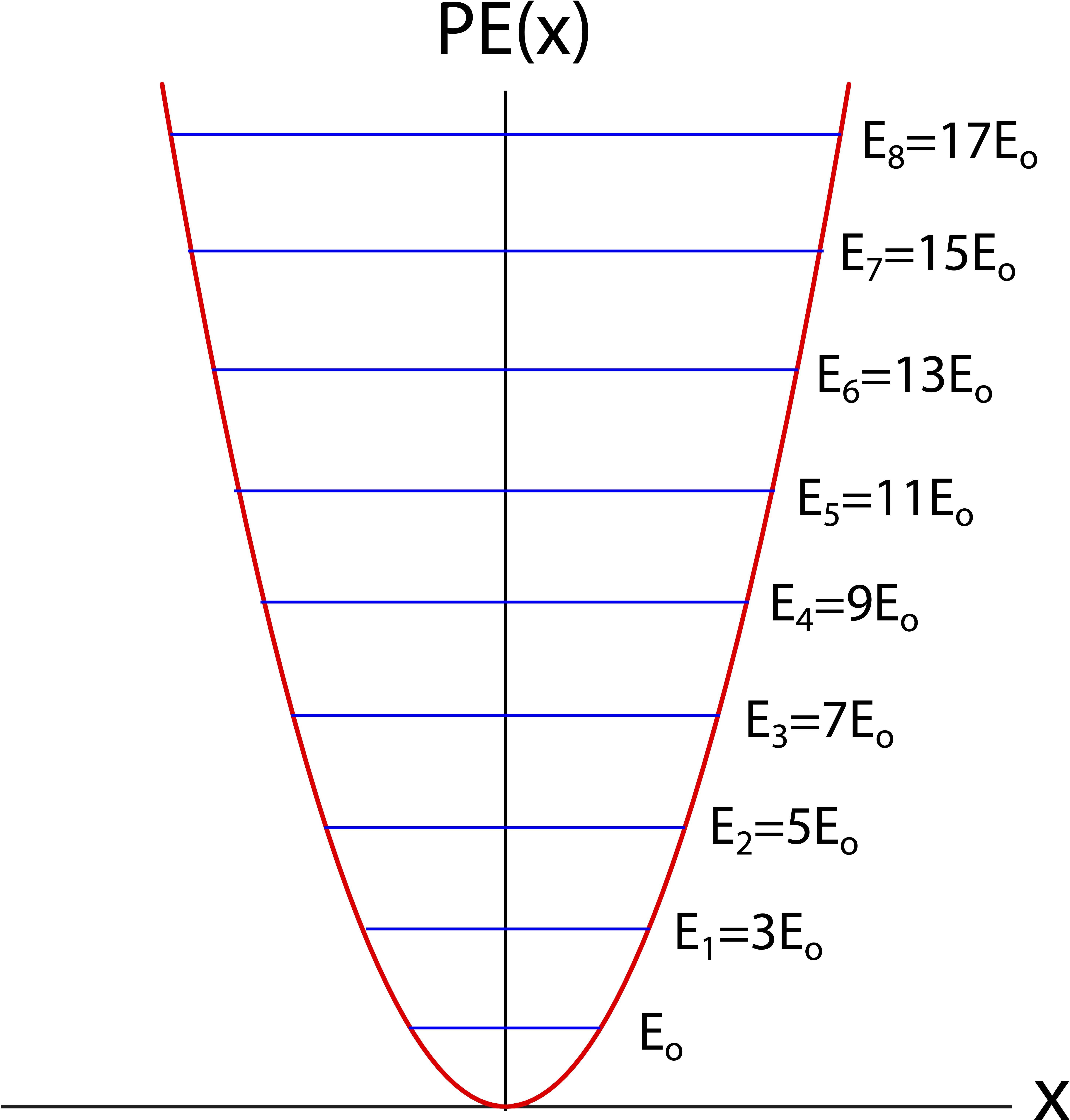
Unlike the case for a one-dimensional infinite box, where the energy level spacing grew with energy, or the hydrogen-like atom, where the energy levels got closer together with increasing energy, for a quantum harmonic oscillator all energy levels are equally spaced. The spacing between two neighboring levels is:
\[E_{n+1}-E_n=2E_o=hf\label{QHO-gap}\]
The quantization of energy also helps us understand the freezing of vibrational modes that we learned about in Physics 7A. Let us consider a diatomic molecule that vibrates at a frequency \(f\). From Physics 7A, recall that the “typical” amount of thermal energy available per mode is \(\frac{1}{2}k_B T\), where \(k_B\) is Boltzmann’s constant, \(1.38 \times 10^{−23} \text{ J/K}\), and \(T\) is the temperature (expressed in Kelvin). For the atoms to vibrate two vibrational modes must be activated – one potential and one kinetic. The amount of thermal energy available to two modes is \(k_B T\). To transfer the system to a higher state, it must gain an amount of energy \(E = hf\) as derived in Equation \ref{QHO-gap}. If the thermal energy \(k_B T\) available is less than \(hf\), then the molecule does not have enough energy to go up an energy level. We say the vibrational modes are frozen out because we cannot transfer energy into them. When the amount of thermal energy is high enough to overcome the gap between energy levels, then energy can transfer into the vibrational energy of the atoms, and we say a vibrational mode has been activated. The thermal energy available per mode is controlled by the value of temperature \(T\).
Example \(\PageIndex{1}\)
Oxygen gas O2 has a vibrational frequency of \(5 \times 10^{13} \text{ Hz}\).
a) Calculate the temperature required to active the vibrational modes of O2.
b) Determine the wavelength of the absorbed photon when the vibrational mode is activated.
- Solution
-
a) To calculate the temperature required to activate vibrational modes, we need to set the energy gap of the quantum harmonic oscillator to the thermal energy of vibrational modes for a diatomic molecule:
\[hf=k_BT\nonumber\]
Solving for temperature:
\[T=\dfrac{hf}{k_B}=\dfrac{6.626\times 10^{-34} J\cdot 5\times 10^{13} Hz}{1.38\times 10^{-23}J/K}=2402 K\nonumber\]
b) The energy gap is equal to the energy of the photon:
\[E_{\text{photon}}=\dfrac{hc}{\lambda}=hf\nonumber\]
The frequency \(f\) in the equation above is the vibrational frequency of O2 and not the frequency of the photon. Solving for the wavelength:
\[\lambda=\dfrac{c}{f}=\dfrac{3\times 10^8 m/s}{5\times 10^{13} Hz}=6\times 10^{-6} m=6000 nm\nonumber\]