3.7: Energy Diagrams

An energy diagram provides us a means to assess features of physical systems at a glance. We will examine a couple of simple examples, and then show how it can be used for more advanced cases in physics and chemistry. It's important to understand that there is no new physics in here – what we have learned so far now is simply represented diagrammatically, making it easier in some cases to see the "big picture" of a physical system.

Elements of Energy Diagrams

First of all, it should be noted that we will be confining ourselves to energy diagrams for 1-dimensional motion. This dimension will be represented by the horizontal axis, and the vertical axis will have units of energy. Secondly, the physical systems represented by energy diagrams will involve only one (conservative) force acting on an object.

Construction of an energy diagram entails first graphing the potential energy function for the conservative force on the axes. Note that potential energy function includes an arbitrary additive constant, which means that the entire graph can be moved up or down on the vertical axis as much as one likes without changing the physical system at all. There is one common convention that is followed regarding the height of the graph on the vertical axis, which we will see below, but it should be remembered that this is only convention, and doesn't change any of the physical properties of the system.

The graph of the potential energy function could apply to any object under the influence of this conservative force. To represent a specific system, the diagram also needs to indicate the total mechanical energy of the system, and this is done with a horizontal line with the correct height on the vertical axis.

That's all there is to drawing these diagrams. The real value comes from interpreting them, which we will discuss in the context of a couple of simple examples.

Two Simple Examples

Let's look at the energy diagrams for the two conservative forces we have dealt with so far... gravity and the elastic force.

Gravity

If we choose the arbitrary constant \(U_o\) for the gravitational potential energy to be zero, we have as a graph of the potential energy function a straight line that passes through the origin. We then include a horizontal line to represent the total energy of the particular system (which I will label as \(E_{tot}\)). Now for interpretation...

Figure 3.7.1 – Energy Diagram for Object Influenced by Gravity Near Earth's Surface

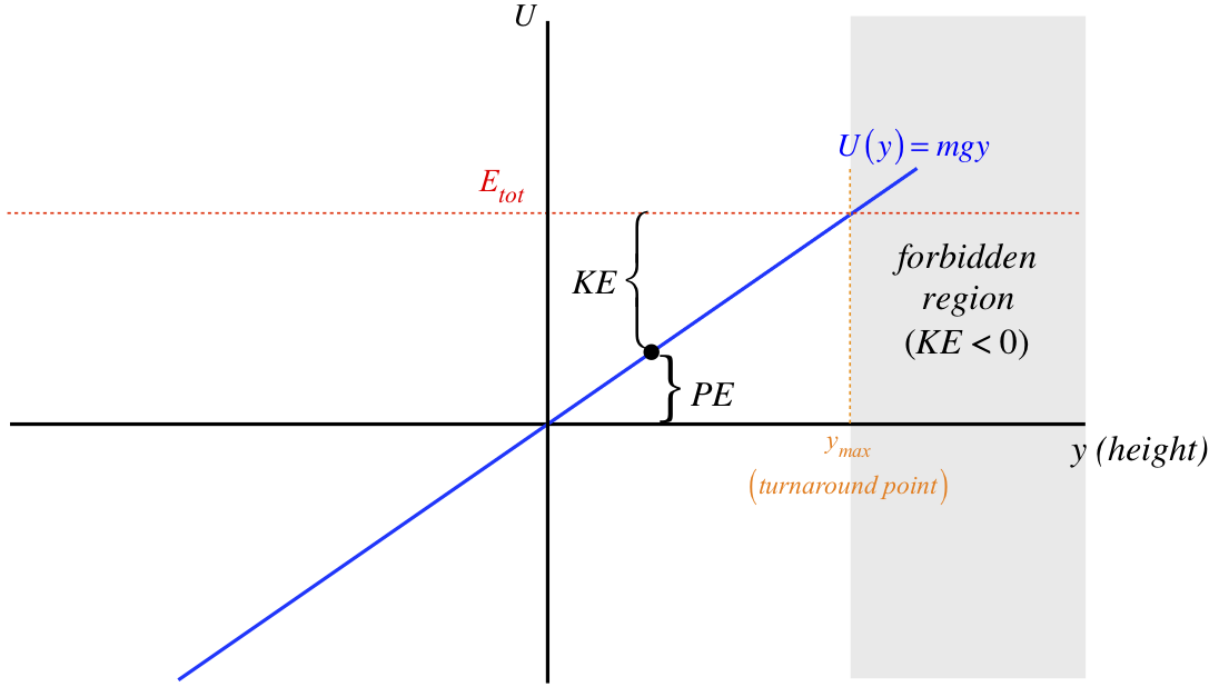
The position of the object (which in this case is the height above some defined zero point), is the value along the horizontal axis. For every position of the object, there is a corresponding value of its potential energy, given by the height of the \(U\left(y\right)\) graph above (if positive) or below (if negative) the horizontal axis. The total (mechanical) energy of this system is conserved (i.e. it is the same for every position of the object), which explains why the total energy graph is a horizontal line. For a given position, the gap between the total energy line and the potential energy line equals the kinetic energy of the object, since the sum of this gap and the height of the potential energy graph is the total energy.

We can also interpret the intersection point of the total energy and the potential energy graphs. At this point, the total energy equals the potential energy, which means the object has no kinetic energy – i.e. the object is at rest at this position. How can an object under the influence of only gravity be at rest? It can be for just an instant, when it reaches the peak of its flight. Therefore the value on the horizontal axis corresponding to this intersection point is the highest elevation the object can reach. Note that for heights (horizontal axis values) greater than this, the potential energy is greater than the mechanical energy, which would require a negative kinetic energy. This is of course impossible, and we call this the forbidden region of the diagram, as we will never find the system in one of these states. As time passes, when the object reaches the intersection point, it must have done so from the allowed region, which means that when the object comes to rest here, is reverses its direction of motion. Consequently, this position is often referred to as the turnaround point.

There is one other nugget of information we can extract from this diagram, though in this particular case it is fairly trivial. If we evaluate the negative of the slope of the potential energy graph at the point where the object is at some moment, we know the force acting on the object at that moment. In the case of gravity, the force is the same everywhere:

\[ F_y = -\dfrac{dU}{dy} = -\dfrac{d}{dy} \left(mgy\right) = -mg \]

[Note: There is no need for partial derivatives here, as we are only dealing with one-dimensional potential energy functions.]

If we change the arbitrary constant, the only quantities that change in the entire picture are the potential energy and total energy. Every physically-observable quantity (kinetic energy, turnaround point, and force) remains unchanged. This may not be immediately apparent, but looking at the graph it is easy to see:

Figure 3.7.2 – Redefined Zero Point for Gravitational Potential Energy

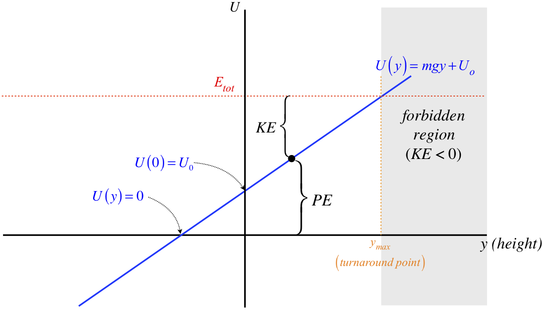
Interestingly, the fact that this potential is a straight line means that a shift of the graph up or down by an additive constant is equivalent to redefining the origin. This is easily seen by noting that this graph can also be viewed as the previous graph shifted to the left by \(y_o\), where \(mgy_o=U_o\). So for this simple case, changing the zero point of potential energy is equivalent to changing the position which we call the origin.

Elastic Force

We take precisely the same steps to draw the energy diagram for a mass on a spring, but there are some differences, such as two forbidden regions and a different slope for every position, and there is one additional feature for this potential that doesn't exist for the case of gravity: an equilibrium point.

Figure 3.7.3 – Energy Diagram for Object Influenced by Elastic Force

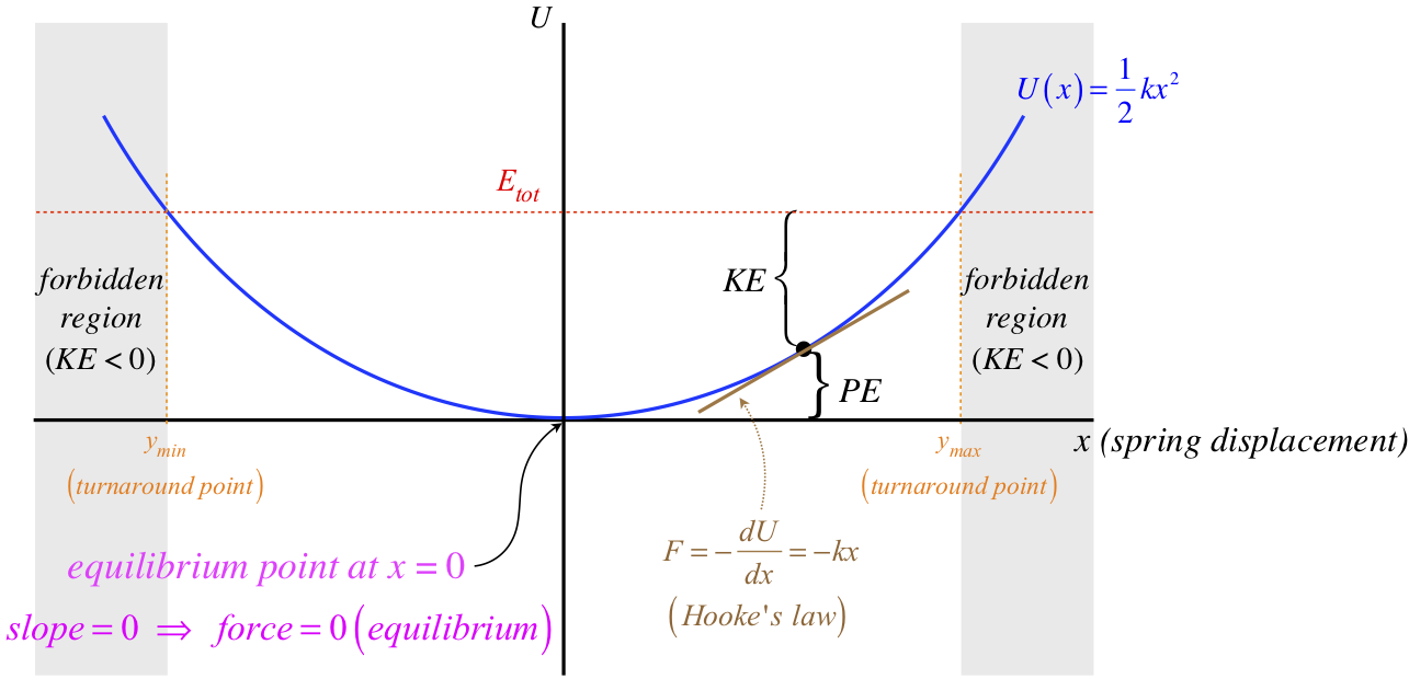
The two forbidden regions arise here because the spring has a maximum stretch and a maximum compression that result in potential energy equaling the total energy. Regions of potential energy confined by two turnaround points like this are often referred to as potential wells. Clearly the slope of the potential energy curve is different everywhere, which reflects the fact that the force by the spring is different for every position the mass can have.

An equilibrium point occurs whenever the slope vanishes (at maxima, minima, and inflection points in the potential energy curve) – there are simply places where the force vanishes. For the spring, it is the position where the spring is neither stretched nor compressed from its natural length. This particular equilibrium is referred to as a stable equilibrium for the following reason: If the object is at rest at this point, and it is given a small nudge in either direction, the resulting force acts to bring the object back to its original position. We can see this here, because the slope on the (+) side of the equilibrium point is positive, which means the force is in the negative direction. The force on the (–) side of the equilibrium point similarly acts back toward the equilibrium. Forces that create stable equilibrium like this are called restoring forces.

It should be clear that any minimum in the potential energy curve will lead to a stable equilibrium, but what about maxima? In this case, the forces that result from small displacements away from the equilibrium point act to push or pull the object farther from its starting point. This type of equilibrium is therefore referred to as an unstable equilibrium. Inflection points lie between parts of the curve that are concave (stable) on one side and convex (unstable) on the other, and the resulting equilibrium is referred to as a meta-stable equilibrium.

As with the case of gravity, shifting the entire curve up or down by an amount \(U_o\) doesn't change any of the physics, including the position of the equilibrium point. Unlike the gravity case, shifting the entire curve left or right (changing the definition of the origin) is not equivalent to the addition of an additive constant to the potential energy curve. But in both cases, the physics is unchanged by the positioning of the curve relative to either of the axes.

Bound States of Two Particles

While our models of terrestrial gravity and the elastic force are useful, we have to keep in mind that force interactions are between two objects, and the energy diagrams we have drawn appear to involve only a single object. The leap to discussing two objects is not a difficult one. Instead of being a position along the \(x\) or \(y\) axis, the one dimension of freedom becomes the separation of the two objects, which we represent with the variable \(r\). If we can express the force as a function of the separation of the two objects interacting, then we can express the potential energy as a function of that variable as well, and voilà – we can draw an energy diagram. For the sake of interpreting such diagrams correctly, we have to keep in mind that the horizontal axis represents a separation, rather than a position, which leads to a big difference from the energy diagrams we created above – the horizontal axis has no negative values. It also should be remembered that these diagrams only relate motion between the particles along the line joining them. If we want to include motion around each other (as in the case of an orbit), we require more information than we can get from the energy diagram.

When we look at the universe in both the microscopic and macroscopic realm, we see countless examples of forces holding systems together. Gravity interactions between the sun and the planets keeps them in orbit. Electromagnetic interactions between protons and electrons holds them together in atoms, and electromagnetic interactions between atoms bind them into molecules. Systems of two bodies that possess too little total energy to escape each other's attractive force are in what is called a bound state. For the purposes of this section, we will confine ourselves to discussing bound states between microscopic particles, and save the discussion of orbits of celestial bodies for the chapter on gravitation.

Bound states between atoms and molecules in our universe are quite extraordinary. Here is how the famous Nobel laureate Richard Feynman put it:

If, in some cataclysm, all of scientific knowledge were to be destroyed, and only one sentence passed on to the next generations of creatures, what statement would contain the most information in the fewest words? All things are made of atoms—little particles that move around in perpetual motion, attracting each other when they are a little distance apart, but repelling upon being squeezed into one another. In that one sentence ... there is an enormous amount of information about the world.

From our earlier discussion, we know that this means that forces between atoms (and between molecules, which are clusters of atoms) must be restoring in nature, with an equilibrium separation. Indeed this does tell us a lot about the shape of the potential energy curve – it must contain a local minimum. But we know even more than this. Clearly a separation distance of zero is not possible (the particles can't occupy the same space), and this is assured by an ever-increasing force as they continue to get closer. This means that the potential energy curve gets steeper and approaches infinity as the separation distance gets closer to zero (i.e. the graph gets closer to the vertical axis). We know one other thing: The force between the two particles gets weaker as they get farther apart, and drops to zero in the limit as their separation goes to infinity. This means that the potential energy curve "flattens out" to a horizontal line as the distance from the vertical axis goes to infinity. Amazingly, this seemingly insignificant amount of information gives us a general shape for the interaction potential of two particles.

Figure 3.7.4 – Shape of Inter-Particle Interaction Potentials

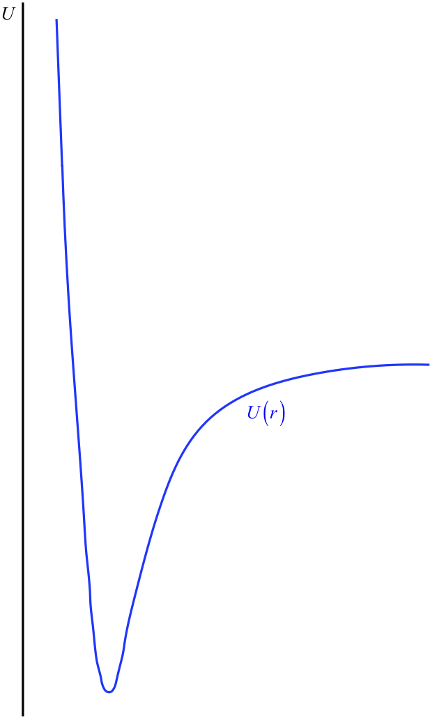
The horizontal axis has been intentionally left out here, because this is not something we can determine. Recall that this potential energy curve can be raised or lowered an arbitrary amount without changing the physics, so we are actually free to place the horizontal axis (the point of zero energy) wherever we like. It is here that we come to the convention alluded-to at the start of this section: It is generally agreed to place the horizontal axis at the position that the potential energy curve reaches as \(r \rightarrow \infty \). That is, it is usually agreed that the potential energy of the interaction vanishes when the particles are separated by an infinite distance (see Figure 3.7.5).

One nice consequence of the \(U\left(r \rightarrow \infty \right) \rightarrow 0\) is that it gives us a simple rule-of-thumb to determine whether or not the two particles in this potential are bound to each other. If the total energy of the system is positive (i.e. the horizontal line representing the total energy is above the \(r\)-axis), then that means that when the two particles are moving away from each other, the graphs never intersect to give a "forbidden region," and they just keep moving apart – they are not bound. If the total energy is negative, then the total energy horizontal line intersects the potential energy graph in two places, giving two turnaround points, keeping the particles within a range of separations.

Figure 3.7.5 – Bound and Unbound States

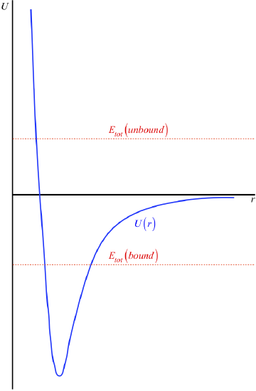
All of the physical interpretations we came up with above apply to this function as well, though it might be a bit confusing at first, since for much of the graph the potential energy is negative. But note:

• The kinetic energy for a specific position is still always positive, and equals the gap between the point on the curve and the total energy line.
• The force between the particles is still the negative of the slope, which means it is attractive (seeks to make \(r\) smaller) when the slope is positive, and is repulsive (seeks to make \(r\) bigger) when the slope is negative.
• The equilibrium and turnaround points are defined as the bottom of the dip and the intersection points of the total energy line and potential energy curve, respectively.

Alert

When two particles are bound to each other, to break the bond, energy must be added to the system. That is, the total energy line must be moved up until it is above the \(r\)-axis. Systems of particles must receive additional energy to break chemical bonds, and energy only comes out of chemical reactions in which new bonds are formed. For some reason, belief of the exact reverse is a very common misconception.

A model of the potential energy that works very well for two neutrally-charged atoms or molecules was constructed in 1924 by John Lennard-Jones. This Lennard-Jones potential has a simple-but-surprising form (yes, those powers are not typos!):

\[ U\left(r \right) = \epsilon \left[ {\left( \dfrac{r_o}{r} \right)}^{12} - 2 {\left( \dfrac{r_o}{r} \right)}^6 \right] \]

Example \(\PageIndex{1}\)

Show that in the Lennard-Jones potential, \(r_o\) is the separation of the particles when they are at equilibrium, and \(\epsilon\) is the depth of the potential well (expressed as a positive value).

Solution

The minimum of this curve occurs at the point where the derivative vanishes, so:

\[ 0 = \dfrac{dU}{dr} = \epsilon \dfrac{d}{dr} \left[ {\left( \dfrac{r_o}{r} \right)}^{12} - 2 {\left( \dfrac{r_o}{r} \right)}^6 \right] = 12{\left( \dfrac{r_o}{r} \right)}^{11} - 12 {\left( \dfrac{r_o}{r} \right)}^5 \;\;\; \Rightarrow \;\;\; r = r_o \nonumber \]

The value of the potential at the minimum is \(U \left(r=r_o \right) \), which one can see from a simple plug-in is in fact equal to \(\left(- \epsilon \right) \).

Example \(\PageIndex{2}\)

A system of two particles bound in a Lennard-Jones potential requires that an addition of energy equal to \(\frac{3}{4}\epsilon\) in order to become unbound. Find the turnaround points of this bound system in terms of \(r_o\).

Solution

The potential energy equals to the total energy at the turnaround points, and the total energy is given to be \(-\frac{3}{4}\epsilon\) (i.e. the energy to unbind the particles is the amount needed to bring the total energy to zero), so:

\[ -\frac{3}{4}\epsilon = \epsilon \left[ {\left( \dfrac{r_o}{r} \right)}^{12} - 2 {\left( \dfrac{r_o}{r} \right)}^6 \right] \;\;\; \Rightarrow \;\;\; -\frac{3}{4}= \left[ x^2 - 2x \right], \;\;\;\;\; where\;\;x \equiv {\left( \dfrac{r_o}{r} \right)}^6 \nonumber \]

Now solve the quadratic for \(x\):

\[ 4x^2 -8x +3 = 0 \;\;\; \Rightarrow \;\;\; x = \dfrac{8 \pm \sqrt{8^2 - 4\left(4\right)\left(3\right)}}{2\left(4\right)} = \frac{3}{2} \;\; or \;\; \frac{1}{2} \nonumber \]

Now solve for the two r values:

\[ {\left( \dfrac{r_o}{r} \right)}^6 = x \;\;\; \Rightarrow \;\;\; r = x^{-\frac{1}{6}} r_o \;\;\; \Rightarrow \;\;\; r_{min}=\boxed{0.93 r_o}, \;\;\; r_{max}=\boxed{1.12 r_o} \nonumber \]

Modeling Bonds as Springs

It is quite common to model chemical bonds as springs, but this seems like a strange practice, given that the potential energy function looks like Equation 3.7.2, which is nothing like the potential energy function of a spring. Surprisingly, a spring can nevertheless act as a reasonable replacement for the Lennard-Jones potential when the total energy is deep in the well. Certainly the curve at the bottom of the well resembles the parabolic curve of the elastic potential, but one might argue that the bottom of any concave curve will resemble the elastic potential energy curve. It turns out that this argument is completely correct – every smooth concave curve can be approximated by the parabolic curve of the elastic potential energy!

How well this approximation works depends upon the range of values we confine ourselves to. If we look at the whole curve, then obviously the approximation of the Lennard-Jones potential with a parabola breaks down badly. But as we narrow-down our view to a smaller and smaller range near the bottom of the well, this approximation gets better.

The reason this works is related to some amazing mathematics: Any smooth function of a single variable can be written as a series (often infinite) of powers of that variable, with each term multiplied by a different constant:

\[ f\left( x \right) = a_o + a_1 x + a_2 x^2 + a_3 x^3 + \dots \]

From this perspective, it's clear that every function has a bit of the \(x^2\) function in it. For the Lennard-Jones potential, we can define \(x\) in the expansion above as \(\left(1-\dfrac{r}{r_o}\right)\), which is a measure of how far the particle separation is from the equilibrium. For example, if the separation distance \(\left(r\right)\) is 90% of the equilibrium distance \(\left(r_o\right)\), then \(\left(1-\dfrac{r}{r_o}\right)=0.1\), and for \(r\) equal to 99% of \(r_o\), \(\left(1-\dfrac{r}{r_o}\right)=0.01\).

In the spring model, it is precisely the distance that the spring is stretched or compressed from the equilibrium that determines the potential energy. So if we write the Lennard-Jones potential as an expansion in powers of \(\left(1-\dfrac{r}{r_o}\right)\), we can more easily compare it to a spring potential energy:

\[ \epsilon \left[ {\left( \dfrac{r_o}{r} \right)}^{12} - 2 {\left( \dfrac{r_o}{r} \right)}^6 \right] = U\left( r \right) = a_o + a_1 \left(1-\dfrac{r}{r_o}\right) + a_2 \left(1-\dfrac{r}{r_o}\right)^2 + a_3 \left(1-\dfrac{r}{r_o}\right)^3 + \dots \]

To use a spring to model this function, we want the series to look like a quadratic, so we need the contributions of the terms in the series with powers greater than 2 to be small compared to the terms before them. Well, if we restrict ourselves to values of \(r\) that are close to \(r_o\) (i.e. consider particles that are separated by a distance close to the equilibrium separation, which means the total energy is quite low), then the difference \(\left(1-\dfrac{r}{r_o}\right)\) is a small number less than 1. The more times we multiply this small number by itself, the smaller the result, so higher powers provide ever-smaller contributions to the sum of the series.

All that remains if we are going to use the elastic potential energy to approximate the Lennard-Jones (or any other) potential is to figure out how to determine the equivalent "spring constant." Fortunately we have a nice trick for doing this. We can compare the way in which the spring constant enters the potential energy function to the series expansion, and determine what number we need from the series expansion to find the effective spring constant:

\[ \frac{1}{2}k_{eff}x^2 = a_2x^2 \;\;\; \Rightarrow \;\;\; k_{eff}=2a_2 \]

Okay, so we know where to find the effective spring constant – we express the actual potential as an infinite series, then look at the constant that multiplies the quadratic term in the expansion, and multiply it by two. But this still means we need to come up with the series... or does it? Consider the following useful mathematical trick: First, take two derivatives of Equation 3.7.3:

\[ f\left( x \right) = a_o + a_1 x + a_2 x^2 + a_3 x^3 + \dots \;\;\; \Rightarrow \;\;\; \dfrac{df}{dx} = 0 + a_1 + 2a_2 x + 3a_3 x^2 + \dots \;\;\; \Rightarrow \;\;\; \dfrac{d^2f}{dx^2} = 0 + 0 + 2a_2 + 6a_3 x + \dots \]

Now evaluate this second derivative at the point \(x=0\). All of the terms after the constant term then vanish, leaving what we are looking for:

\[ \left.\dfrac{d^2f}{dx^2}\right|_{x=0} = 2a_2 = k_{eff} \]

It is left as an exercise for the reader to show that the effective spring constant for the Lennard-Jones potential deep within the well comes out to be: \(72\dfrac{\epsilon}{r_o^2}\). [Note that instead of taking two derivatives with respect to \(x\) and evaluating at \(x=0\), where \(x \equiv 1- \dfrac{r}{r_o}\), we can perhaps more easily do the equivalent calculation of taking the derivatives with respect to \(r\) and evaluate at \(r=r_o\).]