11.13: Two-body kinematics

So far the discussion has been restricted to the center-of-momentum system. Actual scattering measurements are performed in the laboratory frame, and thus it is necessary to transform the scattering angle, energies and cross sections between the laboratory and center-of-momentum coordinate frame. In principle the transformation between the center-of-momentum and laboratory frames is straightforward, using the vector addition of the center-of-mass velocity vector and the center-of-momentum velocity vectors of the two bodies. The following discussion assumes non-relativistic kinematics apply.

In chapter \(2.8\) it was shown that, for Newtonian mechanics, the center-of-mass and center-of-momentum frames of reference are identical. By definition, in the center-of-momentum frame the vector sum of the linear momentum of the incoming projectile, \(p_{P}^{Initial}\) and target, \(p_{T}^{Initial}\) are equal and opposite. That is

\[\mathbf{p}_{P}^{Initial}+\mathbf{p}_{T}^{Initial}=0\label{11.161}\]

Using the center-of-momentum frame, coupled with the conservation of linear momentum, implies that the vector sum of the final momenta of the \(N\) reaction products, \(p_{i}^{Final},\) also is zero. That is

\[\sum_{i=1}^{N}\mathbf{p}_{i}^{Final}=0\label{11.162}\]

An additional constraint is that energy conservation relates the initial and final kinetic energies by

\[\frac{\left( p_{P}^{Initial}\right) ^{2}}{2m_{P}}+\frac{\left( p_{T}^{Initial}\right) ^{2}}{2m_{T}}+Q=\frac{\left( p_{P}^{Final}\right) ^{2} }{2m_{P}}+\frac{\left( p_{T}^{Final}\right) ^{2}}{2m_{T}}\label{11.163}\]

where the \(Q\) value is the energy contributed to the final total kinetic energy by the reaction between the incoming projectile and target. For exothermic reactions, \(Q>0,\) the summed kinetic of the reaction products exceeds the sum of the incoming kinetic energies, while for endothermic reactions, \(Q<0,\) the summed kinetic energy of the reaction products is less than that of the incoming channel.

For two-body kinematics, the following are three advantages to working in the center-of-momentum frame of reference.

1. The two incident colliding bodies are colinear as are the two final bodies.
2. The linear momenta for the two colliding bodies are identical in both the incident channel and the outgoing channel.
3. The total energy in the center-of-momentum coordinate frame is the energy available to the reaction during the collision. The trivial kinetic energy of the center-of-momentum frame relative to the laboratory frame is handled separately.

The kinematics for two-body reactions is easily determined using the conservation of linear momentum along and perpendicular to the beam direction plus the conservation of energy, \ref{11.161}-\ref{11.163}. Note that it is common practice to use the term "center-of-mass" rather than "center-of-momentum" in spite of the fact that, for relativistic mechanics, only the center-of-momentum is a meaningful concept.

General features of the transformation between the center-of-momentum and laboratory frames of reference are best illustrated by elastic or inelastic scattering of nuclei where the two reaction products in the final channel are identical to the incident bodies. Inelastic excitation of an excited state energy of \(\Delta E_{ex}\) in either reaction product corresponds to \(Q=-\Delta E_{exc},\) while elastic scattering corresponds to \(Q=-\Delta E_{exc}=0\).

For inelastic scattering, the conservation of linear momenta for the outgoing channel in the center-of-momentum simplifies to

\[\mathbf{p}_{P}^{Final}+\mathbf{p}_{T}^{Final}=0\]

that is, the linear momenta of the two reaction products are equal and opposite.

Assume that the center-of-momentum direction of the scattered projectile is at an angle \(\vartheta _{cm}^{P}=\vartheta\) relative to the direction of the incoming projectile and that the scattered target nucleus is scattered at a center-of-momentum direction \(\vartheta _{cm}^{T}=\pi -\vartheta\). Elastic scattering corresponds to simple scattering for which the magnitudes of the incoming and outgoing projectile momenta are equal, that is, \(\left\vert p_{P}^{Final}\right\vert =\left\vert p_{P}^{Initial}\right\vert\).

Figure \(\PageIndex{1}\): Vector hodograph of the scattered projectile and target velocities for a projectile, with incident velocity \(v_i\), that is elastically scattered by a stationary target body. The circles show the magnitude of the projectile and target body final velocities in the center of mass. The center-of-mass velocity vectors are shown as dashed lines while the laboratory vectors are shown as solid lines. The left hodograph shows normal kinematics where the projectile mass is less than the target mass. The right hodograph shows inverse kinematics where the projectile mass is greater than the target mass. For elastic scattering \(u_T = u^{\prime}_T\).

Velocities

The transformation between the center-of-momentum and laboratory frames requires knowledge of the particle velocities which can be derived from the linear momenta since the particle masses are known. Assume that a projectile, mass \(m_{P}\), with incident energy \(E_{P}\) in the laboratory frame bombards a stationary target with mass \(m_{T}.\) The incident projectile velocity \(v_{i}\) is given by

\[v_{i}=\sqrt{\frac{2E_{P}}{m_{P}}}\]

The initial velocities in the laboratory frame are taken to be

\[\begin{align} w_{P} &=&v_{i} \tag{Initial Lab velocities} \\ w_{T} &=&0 \notag\end{align}\]

The final velocities in the laboratory frame after the inelastic collision are \[\begin{align} &&w_{P}^{\prime } \tag{Final Lab velocities} \\ &&w_{T}^{\prime } \notag\end{align}\]

In the center-of-momentum coordinate system, equation \((11.2.8)\) implies that the initial center-of-momentum velocities are \[\begin{align} u_{P} &=&v_{i}\frac{m_{T}}{m_{P}+m_{T}} \notag \\ u_{T} &=&v_{i}\frac{m_{P}}{m_{P}+m_{T}}\end{align}\]

It is simple to derive that the final center-of-momentum velocities after the inelastic collision are given by

\[\begin{align} u_{P}^{\prime } &=&\frac{m_{T}}{m_{P}+m_{T}}\sqrt{\frac{2}{m_{P}}\tilde{E}} \notag \\ u_{T}^{\prime } &=&\frac{m_{P}}{m_{P}+m_{T}}\sqrt{\frac{2}{m_{P}}\tilde{E}}\end{align}\]

The energy \(\tilde{E}\) is defined to be given by

\[\tilde{E}=E_{P}+Q(1+\frac{m_{P}}{m_{T}})\]

where \(Q=-\Delta E\) which is the excitation energy of the final excited states in the outgoing channel.

Angles

The angles of the scattered recoils are written as

\[\begin{align} &&\theta _{lab}^{P} \tag{Final laboratory angles} \\ &&\theta _{lab}^{T} \notag\end{align}\]

and

\[\begin{align} \vartheta _{cm}^{P} &=&\vartheta \tag{Final CM angles} \\ \vartheta _{cm}^{T} &=&\pi -\vartheta \notag\end{align}\]

where \(\vartheta\) is the center-of-mass (center-of-momentum) scattering angle.

Figure \(\PageIndex{1}\) shows that the angle relations between the laboratory and center of momentum frames for the scattered projectile are connected by

\[\frac{\sin (\vartheta _{cm}^{P}-\theta _{lab}^{P})}{\sin \theta _{lab}^{P}}= \frac{m_{P}}{m_{T}}\sqrt{\frac{E_{P}}{\tilde{E}}}\equiv \tau \label{11.169}\]

where

\[\tau =\frac{m_{P}}{m_{T}}\frac{1}{\sqrt{1+\frac{Q}{E_{P}}(1+\frac{m_{P}}{ m_{T}})}}=\frac{m_{P}}{m_{T}}\frac{1}{\sqrt{1+\frac{Q}{E_{P}/m_{P}}(\frac{ m_{P}+m_{T}}{m_{P}m_{T}})}}\]

and \(\frac{E_{P}}{m_{P}}\) is the energy per nucleon on the incident projectile.

Equation \ref{11.169} can be rewritten as \[\tan \theta _{lab}^{P}=\frac{\sin \vartheta _{cm}^{P}}{\cos \vartheta _{cm}^{P}+\tau }\]

Another useful relation from Equation \ref{11.169} gives the center-of-momentum scattering angle in terms of the laboratory scattering angle.

\[\vartheta _{cm}^{P}=\sin ^{-1}(\tau \sin \theta _{lab}^{P})+\theta _{lab}^{P}\]

This gives the difference in angle between the lab scattering angle and the center-of-momentum scattering angle. Be careful with this relation since \(\vartheta _{lab}^{P}\) is two-valued for inverse kinematics corresponding to the two possible signs for the solution.

The angle relations between the lab and center-of-momentum for the recoiling target nucleus are connected by

\[\frac{\sin (\vartheta _{cm}^{T}-\theta _{lab}^{T})}{\sin \theta _{lab}^{T}}= \sqrt{\frac{E_{P}}{\tilde{E}}}\equiv \tilde{\tau}\label{11.173}\]

That is

\[\vartheta _{cm}^{T}=\sin ^{-1}(\tilde{\tau}\sin \theta _{lab}^{T})+\theta _{lab}^{T}\]

where \[\tilde{\tau}=\frac{1}{\sqrt{1+\frac{Q}{E_{P}}(1+\frac{m_{P}}{m_{T}})}}=\frac{ 1}{\sqrt{1+\frac{Q}{E_{P}/m_{P}}(\frac{m_{P}+m_{T}}{m_{P}m_{T}})}}\]

Note that \(\tilde{\tau}\) is the same under interchange of the two nuclei at the same incident energy/nucleon, and that \(\tilde{\tau}\) is always larger than or equal to unity since \(Q\) is negative. For elastic scattering \(\tilde{ \tau}=1\) which gives \[\theta _{lab}^{T}=\frac{1}{2}(\pi -\vartheta ) \tag{Recoil lab angle for elastic scattering}\]

For the target recoil Equation \ref{11.173} can be rewritten as \[\tan \theta _{lab}^{T}=\frac{\sin \vartheta _{cm}^{T}}{\cos \vartheta _{cm}^{T}+\tilde{\tau}} \tag{Target lab to CM angle conversion}\]

Figure \(\PageIndex{2}\): The kinematic correlation of the laboratory and center-of-mass scattering angles of the recoiling projectile and target nuclei for scattering for \(4.3\) \(MeV\)/nucleon \(^{104}\)Pd on \(^{208}\)Pb (left) and for the inverse \(4.3\) \(MeV\)/nucleon \(^{208}\)Pb on \(^{104}\)Pd (right). The projectile scattering angles are shown by solid lines while the recoiling target angles are shown by dashed lines. The blue curves correspond to elastic scattering, that is \(Q=0\) while the red curves correspond to inelastic scattering with \(Q = −5\) \(MeV\).

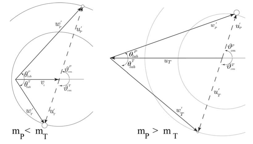
Velocity vector hodographs provide useful insight into the behavior of the kinematic solutions. As shown in Figure \(\PageIndex{1}\), in the center-of-momentum frame the scattered projectile has a fixed final velocity \(u_{P}^{\prime }\), that is, the velocity vector describes a circle as a function of \(\vartheta\). The vector addition of this vector and the velocity of the center-of-mass vector \(-u_{T}\) gives the laboratory frame velocity \(w_{P}^{\prime }\). Note that for normal kinematics, where \(m_{P}<m_{T},\) then \(\left\vert u_{T}\right\vert <\left\vert u_{P}^{\prime }\right\vert\) leading to a monotonic one-to-one mapping of the center-of-momentum angle \(\vartheta _{P}\) and \(\theta _{lab}^{P}\). However, for inverse kinematics, where \(m_{P}>m_{T},\) then \(\left\vert u_{T}\right\vert >\left\vert u_{P}^{\prime }\right\vert\) leading to two valued \(\vartheta\) solutions at any fixed laboratory scattering angle \(\theta\).

Billiard ball collisions are an especially simple example where the two masses are identical and the collision is essentially elastic. Then essentially \(\tau =\tilde{\tau}=1\), \(\theta _{lab}^{P}=\frac{\vartheta _{cm}^{P}}{2},\) and \(\theta _{lab}^{T}=\frac{1}{2}\left( \pi -\vartheta _{cm}^{P}\right)\), that is, the angle between the scattered billiard balls is \(\frac{\pi }{2}\).

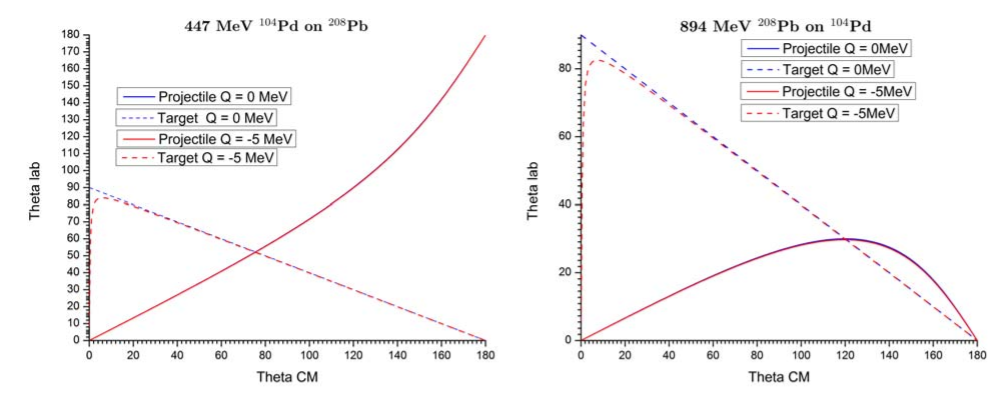
Both normal and inverse kinematics are illustrated in Figure \(\PageIndex{2}\) which shows the dependence of the projectile and target scattering angles in the laboratory frame as a function of center-of-momentum scattering angle for the Coulomb scattering of \(^{104}\)Pd by \(^{208}\)Pb, that is, for a mass ratio of \(2:1\). Both normal and inverse kinematics are shown for the same bombarding energy of \(4.3\) \(MeV/nucleon\) for elastic scattering and for inelastic scattering with a \(Q\)-value of \(-5MeV\).

Figure \(\PageIndex{3}\): Recoil energies, in \(MeV\), versus laboratory scattering angle, shown on the left for scattering of \(447\) \(MeV\) \(^{104}\)Pd by \(^{208}\)Pb with \(Q = −5.0\) \(MeV\), and shown on the right for scattering of \(894\) \(MeV\) \(^{208}\)Pb on \(^{104}\)Pd with \(Q = −5.0\) \(MeV\).

Since \(\sin (\vartheta _{cm}^{T}-\theta _{lab}^{T})\leq 1\) then Equation \ref{11.173} implies that \(\tilde{\tau}\sin \theta _{lab}^{T}\leq 1.\) Since \(\tilde{\tau}\) is always larger than or equal to unity there is a maximum scattering angle in the laboratory frame for the recoiling target nucleus given by

\[\sin \theta _{\max }^{T}=\frac{1}{\tilde{\tau}}\]

For elastic scattering \(\theta _{lab}^{T}=\sin ^{-1}(\frac{1}{\tilde{\tau}} )=90^{\circ }\) since \(\tilde{\tau}=1\) for both \(894\) \(MeV\) \(^{208}\)Pb bombarding \(^{104}\)Pd, and the inverse reaction using a \(447\) \(MeV\) \(^{104}\)Pd beam scattered by a \(^{208}\)Pb target. A \(Q\)-value of \(-5\) \(MeV\) gives\(\ \tilde{\tau}=1.002808\) which implies a maximum scattering angle of \(\theta _{lab}^{T}=85.71^{\circ }\) for both \(894\) \(MeV\) \(^{208}\)Pb bombarding \(^{104}\) Pd, and the inverse reaction of a \(447\) \(MeV\) \(^{104}\)Pd beam scattered by a \(^{208}\)Pb target. As a consequence there are two solutions for \(\vartheta _{cm}^{T}\) for any allowed value of \(\theta _{lab}^{T}\) as illustrated in Figure \(11.13.3\).

Since \(\sin (\vartheta _{cm}^{P}-\theta _{lab}^{P})\leq 1\) then equation \((11.12.18)\) implies that \(\tau \sin \theta _{lab}^{P}\leq 1.\) For a \(447\) \(MeV\) \(^{104}\)Pd beam scattered by a \(^{208}\)Pb target \(\frac{m_{P}}{m_{T}}=0.50\), thus \(\tau =0.5\) for elastic scattering which implies that there is no upper bound to \(\theta _{lab}^{P}\). This leads to a one-to-one correspondence between \(\theta _{lab}^{P}\) and \(\vartheta _{cm}^{P}\) for normal kinematics. In contrast, the projectile has a maximum scattering angle in the laboratory frame for inverse kinematics since \(\frac{m_{P}}{m_{T}}=2.0\) leading to an upper bound to \(\theta _{lab}^{P}\) given by

\[\sin \theta _{\max }^{P}=\frac{1}{\tau }\]

For elastic scattering \(\tau =2\) implying \(\theta _{\max }^{P}=30^{\circ }\). In addition to having a maximum value for \(\theta _{lab}^{P}\), when \(\tau >1,\) also there are two solutions for \(\vartheta _{cm}^{P}\) for any allowed value of \(\theta _{lab}^{P}\). For the example of \(894\) \(MeV\) \(^{208}\)Pb bombarding \(^{178}\)Hf leads to a maximum projectile scattering angle of \(\theta _{lab}^{P}=30.0^{\circ }\) for elastic scattering and \(\theta _{lab}^{P}=29.907^{\circ }\) for \(Q=-5\) \(MeV.\)

Kinetic energies

The initial total kinetic energy in the center-of-momentum frame is

\[E_{cm}^{Initial}=E_{P} \frac{m_{T}}{m_{P}+m_{T}}\]

The final total kinetic energy in the center-of-momentum frame is \[E_{cm}^{Final}=E_{cm}^{Initial}+Q=\tilde{E}\frac{m_{T}}{m_{P}+m_{T}}\]

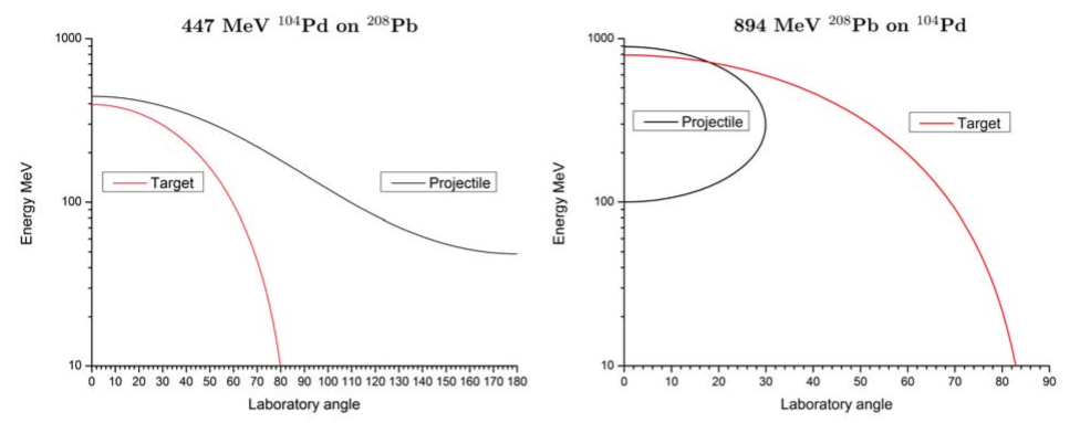
In the laboratory frame the kinetic energies of the scattered projectile and recoiling target nucleus are given by

\[\begin{align} E_{P}^{Lab} &=&\left( \frac{m_{T}}{m_{P}+m_{T}}\right) ^{2}\left( 1+\tau ^{2}+2\tau \cos \vartheta _{cm}^{P}\right) \tilde{E} \\ E_{T}^{Lab} &=&\frac{m_{P}m_{T}}{\left( m_{P}+m_{T}\right) ^{2}}\left( 1+ \tilde{\tau}^{2}+2\tilde{\tau}\cos \vartheta _{cm}^{T}\right) \tilde{E}\end{align}\]

where \(\vartheta _{cm}^{P}\) and \(\vartheta _{cm}^{T}\) are the center-of-mass scattering angles respectively for the scattered projectile and target nuclei.

For the chosen incident energies the normal and inverse reactions give the same center-of-momentum energy of \(298\) \(MeV\) which is the energy available to the interaction between the colliding nuclei. However, the kinetic energy of the center-of-momentum is \(447-298=149\) \(MeV\) for normal kinematics and \(894-298=596\) \(MeV\) for inverse kinematics. This trivial center-of-momentum kinetic energy does not contribute to the reaction. Note that inverse kinematics focusses all the scattered nuclei into the forward hemisphere which reduces the required solid angle for recoil-particle detection.

Solid angles

The laboratory-frame solid angles for the scattered projectile and target are taken to be \(d\omega _{P}\) and \(d\omega _{T}\) respectively, while the center-of-momentum solid angles are \(d\Omega _{P}\) and \(d\Omega _{T}\) respectively. The Jacobian relating the solid angles is \[\frac{d\omega _{P}}{d\Omega _{P}}=\left( \frac{\sin \theta _{lab}^{P}}{\sin \vartheta _{cm}^{P}}\right) ^{2}\left\vert \cos (\vartheta _{cm}^{P}-\theta _{lab}^{P})\right\vert\]

\[\frac{d\omega _{T}}{d\Omega _{T}}=\left( \frac{\sin \theta _{lab}^{T}}{\sin \vartheta _{cm}^{T}}\right) ^{2}\left\vert \cos (\vartheta _{cm}^{T}-\theta _{lab}^{T})\right\vert\]

These can be used to transform the calculated center-of-momentum differential cross sections to the laboratory frame for comparison with measured values. Note that relative to the center-of-momentum frame, the forward focussing increases the observed differential cross sections in the forward laboratory frame and decreases them in the backward hemisphere.

Exploitation of two-body kinematics

Computing the above non-trivial transform relations between the center-of-mass and laboratory coordinate frames for two-body scattering is used extensively in many fields of physics. This discussion has assumed non-relativistic two-body kinematics. Relativistic two-body kinematics encompasses non-relativistic kinematics as discussed in chapter \(17.4\). Many computer codes are available that can be used for making either non-relativistic or relativistic transformations.

It is stressed that the underlying physics for two interacting bodies is identical irrespective of whether the reaction is observed in the center-of-mass or the laboratory coordinate frames. That is, no new physics is involved in the kinematic transformation. However, the transformation between these frames can dramatically alter the angles and velocities of the observed scattered bodies which can be beneficial for experimental detection. For example, in heavy-ion nuclear physics the projectile and target nuclei can be interchanged leading to very different velocities and scattering angles in the laboratory frame of reference. This can greatly facilitate identification and observation of the velocities vectors of the scattered nuclei. In high-energy physics it is advantageous to collide beams having identical, but opposite, linear momentum vectors, since then the laboratory frame is the center-of-mass frame, and the energy required to accelerate the colliding bodies is minimized.