
11.8: Transmission Line with Losses
( \newcommand{\kernel}{\mathrm{null}\,}\)
The voltage and current on a lossless transmission line must satisfy the following equations:
∂2V∂z2=ϵμ0∂2V∂t2,∂2I∂z2=ϵμ0∂2I∂t2.
These are a direct consequence of Maxwell’s equations. Strictly speaking, they are only correct providing that ϵ, the dielectric constant, is truly a constant and therefore independent of frequency. Even the best of dielectric insulating materials exhibit some losses that are frequency dependent: in many cases the imaginary part of the dielectric constant is proportional to the frequency. For a time dependence exp (iωt) the above two equations, (11.8.1), become
∂2V∂z2=−ϵμ0ω2V,∂2I∂z2=−ϵμ0ω2I,
where ϵ may have real and imaginary parts, both of which will depend upon the frequency. Solutions of Equations (11.8.3) that are harmonic in space, i.e. V and I are proportional to exp (−ikz), must be described by a wave-vector k that satisfies the condition
k2=ϵμ0ω2,
In the presence of dielectric losses ϵ will in general be a complex quantity, and therefore so also must the wave-vector be complex :
k=±ω√ϵμ0
so that
k=±(k1−ik2).
The general solutions of the wave equations (11.8.3) for the voltage and current on the transmission line in the presence of a lossy dielectric can be written
V(z,t)=[aexp(−k2z)exp(−ik1z)+bexp(k2z)exp(ik1z)]⋅exp(iωt),I(z,t)=1Z0[aexp(−k2z)exp(−ik1z)−bexp(k2z)exp(ik1z)]exp(iωt),
where (k2/k1) ≪ 1 for a high quality cable, and k1, k2 are the real and imaginary parts of the wave-vector. Notice that k2 must be positive in order that the amplitude of the forward propagating wave decays with distance.
In actual fact, part of the energy loss as a wave propagates down a transmission line is due to Ohmic losses in the skin-depth of the conductors: i.e. the metal electrodes do possess a finite conductivity and therefore there are energy losses due to the shielding currents that flow in them. It can be easily shown, using the methods of Chapter(10), that the rate of energy loss in each conductor per unit area of surface is given by
<Sn>=12√ωμ02σ0|H0|2 Watts /m2.
< Sn > is the time averaged Poynting vector component corresponding to energy flow into the conductor surface, σ0 is the dc conductivity of the metal wall, H0 is the magnetic field strength at the conductor surface, and ω = 2πf is the circular frequency. This energy loss must be added to the energy loss in the dielectric material. The conductor losses can be taken into account by increasing the imaginary part of the wave-vector, k2, in Equations (11.8.5). One can write
V(z,t)=[aexp(−αz)exp(−ik1z)+bexp(αz)exp(+ik1z)]exp(iωt)I(z,t)=1Z0[aexp(−αz)exp(−ik1z)−bexp(αz)exp(+ik1z)]exp(iωt)
where α is an empirical parameter whose frequency dependence can be measured for a particular cable. The constants a,b in (11.8.11) must be adjusted to satisfy the boundary condition at the position of the load; i.e. at the load ZL= V/I. For a cable having a characteristic impedance Z0 that connects a generator at z=0 with a load at z=L this condition requires
ZLZ0=[aexp(−αL)exp(−ik1L)+bexp(αL)exp(ik1L)aexp(−αL)exp(−ik1L)−bexp(αL)exp(ik1L)],
from which
ba=[ZL−1Z0−1]exp(−2αL)exp(−2ik1L).
Using the previous notation zL = ZL/Z0, and zG = ZG/Z0, and
Γ=zL−1zL+1=|Γ|exp(iθ),
one finds
zG=[1+Γexp(−2αL)exp(−2ik1L)1−Γexp(−2αL)exp(−2ik1L)].
Equation (???) shows that the impedance seen by the generator approaches the characteristic impedance of the cable if the load is connected to the generator through a cable that is long compared with the attenuation length (1/α).
Characteristics for a few representative co-axial cables are listed in Table(11.8.1), and their attenuation lengths at a number of frequencies are listed in Table(11.8.2). The length of cable for which the amplitude of a voltage pulse is attenuated to (1/e)= 0.368 of its original amplitude is given by (1/α). For example, this attenuation length is 9.8 meters for RG-8 cable at 5 GHz.
The attenuation parameter, α, for the cables listed in Table(11.8.2) are observed to be approximately proportional to √ω, and this suggests that most of the losses in these cables is due to eddy currents in the conductors.
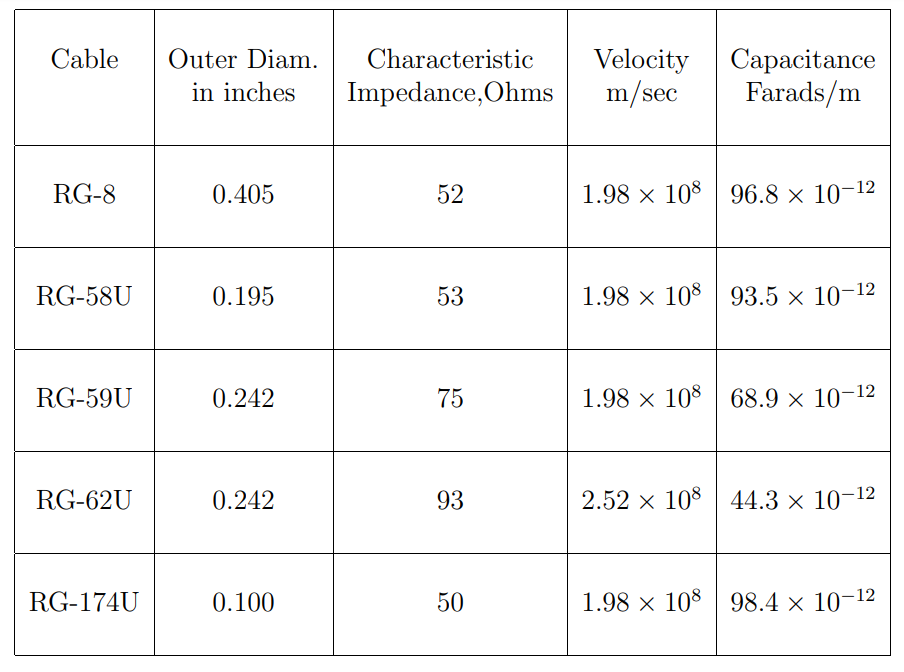
Table 11.8.1: Characteristics of some commonly used commercial co-axial cables. The dielectric material between the conductors is polyethylene. The data was taken from the 1985/86 catalogue of RAE Industrial Electronics Ltd., Vancouver, BC.
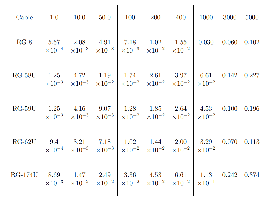
Table 11.8.2: Frequency dependence of the attenuation parameter α for some selected co-axial cables. V(z) = V0 exp (−αz). Frequencies in MHz. The data is taken from the 1985/86 catalogue of RAE Industrial Electronics Ltd., Vancouver, BC.