7.6: Waveguides- H and E Waves

Let us now return to Eqs. (100) and explore the H- and E-waves – with, respectively, either \(\ H_{z}\) or \(\ E_{z}\) different from zero. At the first sight, they may seem more complex. However, Eqs. (101), which determine the distribution of these longitudinal components over the cross-section, are just the 2D Helmholtz equations for scalar functions. For simple cross-section geometries, they may be readily solved using the methods discussed for the Laplace equation in Chapter 2, in particular the variable separation. After the solution of such an equation has been found, the transverse components of the fields may be calculated by differentiation, using the simple formulas,

\[\ \mathbf{E}_{t}=\frac{i}{k_{t}^{2}}\left[k_{z} \nabla_{t} E_{z}-k Z\left(\mathbf{n}_{z} \times \nabla_{t} H_{z}\right)\right], \quad \mathbf{H}_{t}=\frac{i}{k_{t}^{2}}\left[k_{z} \nabla_{t} H_{z}+\frac{k}{Z}\left(\mathbf{n}_{z} \times \nabla_{t} E_{z}\right)\right],\tag{7.121}\]

which follow from the two equations in the first line of Eqs. (100).⁵²

In comparison with the boundary problems of electro- and magnetostatics, the only conceptually new feature of Eqs. (101) is that they form the so-called eigenproblems, with typically many solutions (eigenfunctions), each describing a specific wave mode, and corresponding to a specific eigenvalue of the parameter \(\ k_{t}\). The good news here is that these values of \(\ k_{t}\) are determined by this 2D boundary problem and hence do not depend on \(\ k_{z}\). As a result, the dispersion law \(\ \omega\left(k_{z}\right)\) of any mode, which follows from the last form of Eq. (102),

\[\ \text{Universal dispersion relation}\quad\quad\quad\quad \omega=\left(\frac{k_{z}^{2}+k_{t}^{2}}{\varepsilon \mu}\right)^{1 / 2} \equiv\left(\nu^{2} k_{z}^{2}+\omega_{\mathrm{c}}^{2}\right)^{1 / 2},\tag{7.122}\]

is functionally similar for all modes. It is also similar to that of plane waves in plasma (see Eq. (38), Fig. 6, and their discussion in Sec. 2), with the only differences that the speed in light \(\ c\) is generally replaced with \(\ \nu=1 /(\varepsilon \mu)^{1 / 2}\), i.e. the speed of the plane (or any TEM) waves in the medium filling the waveguide, and that \(\ \omega_{\mathrm{p}}\) is replaced with the so-called cutoff frequency

\[\ \omega_{\mathrm{c}} \equiv \nu k_{t},\tag{7.123}\]

specific for each mode. (As Eq. (101) implies, and as we will see from several examples below, \(\ k_{t}\) has the order of \(\ 1 / a\), where \(\ a\) is the characteristic dimension of waveguide’s cross-section, so that the critical value of the free-space wavelength \(\ \lambda \equiv 2 \pi c / \omega\) is of the order of \(\ a\).) Below the cutoff frequency of each particular mode, such wave cannot propagate in the waveguide.⁵³ As a result, the modes with the lowest values of \(\ \omega_{\mathrm{c}}\) present special practical interest, because the choice of the signal frequency \(\ \omega\) between the two lowest values of the cutoff frequency (123) guarantees that the waves propagate in the form of only one mode, with the lowest \(\ k_{t}\). Such a choice enables engineers to simplify the excitation of the desired mode by wave generators, and to avoid the parasitic transfer of electromagnetic wave energy to undesirable modes by (virtually unavoidable) small inhomogeneities of the system.

The boundary conditions for the Helmholtz equations (101) depend on the propagating wave type. For the \(\ E\)-modes, with \(\ H_{z}=0\) but \(\ E_{z} \neq 0\), the condition \(\ E_{\tau}=0\) immediately gives

\[\ \left.E_{z}\right|_{C}=0,\tag{7.124}\]

where \(\ C\) is the inner contour limiting the conducting wall’s cross-section. For the \(\ H\)-modes, with \(\ E_{z}=0\) but \(\ H_{z} \neq 0\), the boundary condition is slightly less obvious and may be obtained using, for example, the second equation of the system (100), vector-multiplied by \(\ \mathbf{n}_{z}\). Indeed, for the component normal to the conductor surface, the result of such multiplication is

\[\ i k_{z}\left(\mathbf{H}_{t}\right)_{n}-i \frac{k}{Z}\left(\mathbf{n}_{z} \times \mathbf{E}_{t}\right)_{n}=\frac{\partial H_{z}}{\partial n}.\tag{7.125}\]

But the first term on the left-hand side of this relation must be zero on the wall surface, because of the second of Eqs. (104), while according to the first of Eqs. (104), the vector \(\ \mathbf{E}_{t}\) in the second term cannot have a component tangential to the wall. As a result, the vector product in that term cannot have a normal component, so that the term should equal zero as well, and Eq. (125) is reduced to

\[\ \left.\frac{\partial H_{z}}{\partial n}\right|_{C}=0.\tag{7.126}\]

Let us see how does all this machinery work for a simple but practically important case of a metallic-wall waveguide with a rectangular cross-section – see Fig. 22

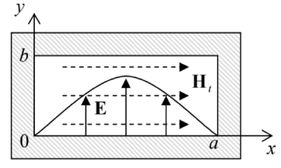Fig. 7.22. A rectangular waveguide, and the transverse field distribution in its fundamental mode \(\ H_{10}\) (schematically).

In the natural Cartesian coordinates, shown in this figure, both Eqs. (101) take the simple form

\[\ \left(\frac{\partial^{2}}{\partial x^{2}}+\frac{\partial^{2}}{\partial y^{2}}+k_{t}^{2}\right) f=0, \quad \text { where } f= \begin{cases}E_{z}, & \text { for } E-\text { modes, } \\ H_{z}, & \text { for } H-\text { modes. }\end{cases}\tag{7.127}\]

From Chapter 2 we know that the most effective way of solution of such equations in a rectangular region is the variable separation, in which the general solution is represented as a sum of partial solutions of the type

\[\ f=X(x) Y(y).\tag{7.128}\]

Plugging this expression into Eq. (127), and dividing each term by \(\ XY\), we get the equation,

\[\ \frac{1}{X} \frac{d^{2} X}{d x^{2}}+\frac{1}{Y} \frac{d^{2} Y}{d y^{2}}+k_{t}^{2}=0,\tag{7.129}\]

which should be satisfied for all values of \(\ x\) and \(\ y\) within the waveguide’s interior. This is only possible if each term of the sum equals a constant. Taking the \(\ X\)-term and \(\ Y\)-term constants in the form \(\ \left(-k_{x}^{2}\right)\) and \(\ \left(-k_{y}^{2}\right)\), respectfully, and solving the corresponding ordinary differential equations,⁵⁴ for the eigenfunction (128) we get

\[\ f=\left(c_{x} \cos k_{x} x+s_{x} \sin k_{x} x\right)\left(c_{y} \cos k_{y} y+s_{y} \sin k_{y} y\right), \quad \text { with } k_{x}^{2}+k_{y}^{2}=k_{t}^{2},\tag{7.130}\]

where the constants \(\ c\) and \(\ s\) should be found from the boundary conditions. Here the difference between the \(\ H\)-modes and \(\ E\)-modes comes in.

For the \(\ H\)-modes, Eq. (130) is valid for \(\ H_{z}\), and we should use the boundary condition (126) on all metallic walls of the waveguide, i.e. at \(\ x=0\) and \(\ a\); and \(\ y=0\) and \(\ b\) – see Fig. 22. As a result, we get very simple expressions for eigenfunctions and eigenvalues:

\[\ \left(H_{z}\right)_{n m}=H_{l} \cos \frac{\pi n x}{a} \cos \frac{\pi m y}{b},\tag{7.131}\]

\[\ k_{x}=\frac{\pi n}{a}, \quad k_{y}=\frac{\pi m}{b}, \quad \text { so that }\left(k_{t}\right)_{n m}=\left(k_{x}^{2}+k_{y}^{2}\right)^{1 / 2}=\pi\left[\left(\frac{n}{a}\right)^{2}+\left(\frac{m}{b}\right)^{2}\right]^{1 / 2},\tag{7.132}\]

where \(\ \mathrm{H}_l\) is the longitudinal field’s amplitude, and \(\ n\) and \(\ m\) are two integer numbers – arbitrary besides that they cannot be equal to zero simultaneously.⁵⁵ Assuming, just for certainty, that \(\ a \geq b\) (as shown in Fig. 22), we see that the lowest eigenvalue of \(\ k_t\), and hence the lowest cutoff frequency (123), is achieved for the so-called \(\ H_{10}\) mode with \(\ n = 1\) and \(\ m = 0\), and hence with

\[\ \text{Fundamental mode’s cutoff}\quad\quad\quad\quad \left(k_{t}\right)_{10}=\frac{\pi}{a},\tag{7.133}\]

thus confirming our prior estimate of \(\ k_{t}\).

Depending on the \(\ a/b\) ratio, the second-lowest \(\ k_{t}\) (and hence \(\ \omega_{\mathrm{c}}\)) belongs to either the \(\ H_{11}\) mode with \(\ n = 1\) and \(\ m = 1\):

\[\ \left(k_{t}\right)_{11}=\pi\left(\frac{1}{a^{2}}+\frac{1}{b^{2}}\right)^{1 / 2} \equiv\left[1+\left(\frac{a}{b}\right)^{2}\right]^{1 / 2}\left(k_{t}\right)_{10},\tag{7.134}\]

or to the \(\ H_{20}\) mode with \(\ n = 2\) and \(\ m = 0\):

\[\ \left(k_{t}\right)_{20}=\frac{2 \pi}{a} \equiv 2\left(k_{t}\right)_{10}.\tag{7.135}\]

These values become equal at \(\ a / b=\sqrt{3} \approx 1.7\); in practical waveguides, the \(\ a/b\) ratio is not too far from this value. For example, in the standard X-band \(\ (\sim 10-\mathrm{GHz})\) waveguide WR90, \(\ a \approx 2.3 \mathrm{~cm}\) \(\ (f_{\mathrm{c}} \equiv \omega_{\mathrm{c}} / 2 \pi \approx6.5 \text{ GHz})\), and \(\ b \approx 1.0 \mathrm{~cm}\).

Now let us have a look at the alternative \(\ E\)-modes. For them, we still should use the general solution (130) with \(\ f=E_{z}\), but now with the boundary condition (124). This gives us the eigenfunctions

\[\ \left(E_{z}\right)_{n m}=E_{l} \sin \frac{\pi n x}{a} \sin \frac{\pi m y}{b},\tag{7.136}\]

and the same eigenvalue spectrum (132) as for the H modes. However, now neither \(\ n\) nor \(\ m\) can be equal to zero; otherwise Eq. (136) would give the trivial solution \(\ E_{z}(x, y)=0\). Hence the lowest cutoff frequency of TM waves is achieved at the so-called \(\ E_{11}\) mode with \(\ n =1\), \(\ m = 1\), and with the eigenvalue given by Eq. (134), always higher than \(\ \left(k_{t}\right)_{10}\).

Thus the fundamental \(\ H_{10}\) mode is certainly the most important wave in rectangular waveguides; let us have a better look at its field distribution. Plugging the corresponding solution (131) with \(\ n = 1\) and \(\ m = 0\) into the general relation (121), we easily get

\[\ \left(H_{x}\right)_{10}=-i \frac{k_{z} a}{\pi} H_{l} \sin \frac{\pi x}{a}, \quad\left(H_{y}\right)_{10}=0,\tag{7.137}\]

\[\ \left(E_{x}\right)_{10}=0, \quad\left(E_{y}\right)_{10}=i \frac{k a}{\pi} Z H_{l} \sin \frac{\pi x}{a}.\tag{7.138}\]

This field distribution is (schematically) shown in Fig. 22. Neither of the fields depends on the coordinate y – the feature very convenient, in particular, for microwave experiments with small samples. The electric field has only one (in Fig. 22, vertical) component that vanishes at the side walls and reaches its maximum at the waveguide’s center; its field lines are straight, starting and ending on wall surface charges (whose distribution propagates along the waveguide together with the wave). In contrast, the magnetic field has two non-zero components (\(\ H_{x}\) and \(\ H_{z}\)), and its field lines are shaped as horizontal loops wrapped around the electric field maxima.

An important question is whether the \(\ H_{10}\) wave may be usefully characterized by a unique impedance introduced similarly to \(\ Z_{W}\) of the TEM modes – see Eq. (115). The answer is not, because the main value of \(\ Z_{W}\) is a convenient description of the impedance matching of a transmission line with a lumped load – see Fig. 19 and Eq. (118). As was discussed above, such a simple description is possible (i.e., does not depend on the exact geometry of the connection) only if both dimensions of the line’s cross-section are much less than \(\ \lambda\). But for the \(\ H_{10}\) wave (and more generally, any non-TEM mode) this is impossible – see, e.g., Eq. (129): its lowest frequency corresponds to the TEM wavelength \(\ \lambda_{\max}=2 \pi /\left(k_{t}\right)_{\min }=2 \pi /\left(k_{t}\right)_{10}=2 a\). (The reader is challenged to find a simple interpretation of this equality.)

Now let us consider metallic-wall waveguides with a round cross-section (Fig. 23a). In this single-connected geometry, the TEM waves are impossible again, while for the analysis of \(\ H\)-modes and \(\ E\)-modes, the polar coordinates \(\ \{\rho, \varphi\}\) are most natural. In these coordinates, the 2D Helmholtz equation (101) takes the following form:

\[\ \left[\frac{1}{\rho} \frac{\partial}{\partial \rho}\left(\rho \frac{\partial}{\partial \rho}\right)+\frac{1}{\rho^{2}} \frac{\partial^{2}}{\partial \varphi^{2}}+k_{t}^{2}\right] f=0, \quad \text { where } f= \begin{cases}E_{z}, & \text { for } E \text { - modes, } \\ H_{z}, & \text { for } H \text { - modes. }\end{cases}\tag{7.139}\]

Separating the variables as \(\ f=\mathcal{R}(\rho) \mathcal{F}(\varphi)\), we get

\[\ \frac{1}{\rho \mathcal{R}} \frac{d}{d \rho}\left(\rho \frac{d \mathcal{R}}{d \rho}\right)+\frac{1}{\rho^{2} \mathcal{F}} \frac{d^{2} \mathcal{F}}{d \varphi^{2}}+k_{t}^{2}=0.\tag{7.140}\]

But this is exactly the Eq. (2.127) that was studied in Sec. 2.7 in the context of electrostatics, just with a replacement of notation: \(\ \gamma \rightarrow k_{t}\). So we already know that to have \(\ 2 \pi\)-periodic functions \(\ \mathcal{F}(\varphi)\) and finite values \(\ \mathcal{R}(0)\) (which are evidently necessary for our current case – see Fig. 23a), the general solution must have the form given by Eq. (2.136), i.e. the eigenfunctions are expressed via integer-order Bessel functions of the first kind:

\[\ f_{n m}=J_{n}\left(k_{n m} \rho\right)\left(c_{n} \cos n \varphi+s_{n} \sin n \varphi\right) \equiv \operatorname{const} \times J_{n}\left(k_{n m} \rho\right) \cos n\left(\varphi-\varphi_{0}\right),\tag{7.141}\]

with the eigenvalues \(\ k_{n m}\) of the transverse wave number \(\ k_{t}\) to be determined from appropriate boundary conditions, and an arbitrary constant \(\ \varphi_{0}\).

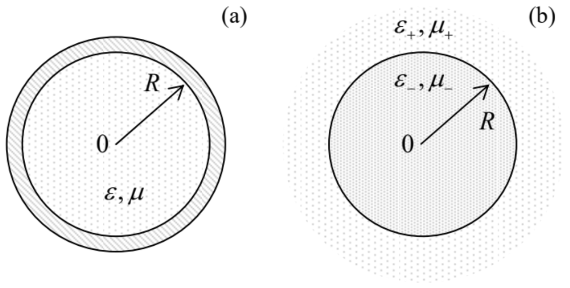Fig. 7.23. (a) Metallic and (b) dielectric waveguides with circular cross-sections.

As for the rectangular waveguide, let us start from the \(\ H\)-modes \(\ \left(f=H_{z}\right)\). Then the boundary condition on the wall surface \(\ (\rho=R)\) is given by Eq. (126), which, for the solution (141), takes the form

\[\ \frac{d}{d \xi} J_{n}(\xi)=0, \quad \text { where } \xi \equiv k R.\tag{7.142}\]

This means that eigenvalues of Eq. (139) are

\[\ k_{t}=k_{n m}=\frac{\xi_{n m}^{\prime}}{R},\tag{7.143}\]

where \(\ \xi_{n m}^{\prime}\) is the \(\ m^{\text {th }}\) zero of the function \(\ d J_{n}(\xi) / d \xi\). Approximate values of these zeros for several lowest \(\ n\) and \(\ m\) may be read out from Fig. 2.18; their more accurate values are given in Table 1 below.

Table 7.1. Zeros \(\ \xi^{\prime}{ }_{n m}\) of the function \(\ d J_{n}(\xi) / d \xi\) for a few lowest values of the Bessel function’s index \(\ n\) and the root’s number \(\ m\).

	\(\ m = 1\)	2	3
\(\ n = 0\)	3.83171	7.015587	10.1735
1	1.84118	5.33144	8.53632
2	3.05424	6.70613	9.96947
3	4.20119	8.01524	11.34592

The table shows, in particular, that the lowest of the zeros is \(\ \xi^{\prime}{ }_{11} \approx 1.84\).⁵⁶ Thus, perhaps a bit counter-intuitively, the fundamental mode, providing the lowest cutoff frequency \(\ \omega_{\mathrm{c}}=\nu k_{n m}\), is \(\ H_{11}\), corresponding to \(\ n = 1\) rather than \(\ n = 0\):

\[\ H_{z}=H_{l} J_{1}\left(\xi_{11}^{\prime} \frac{\rho}{R}\right) \cos \left(\varphi-\varphi_{0}\right).\tag{7.144}\]

It has the transverse wave number is \(\ k_{t}=k_{11}=\xi_{11}^{\prime} / R \approx 1.84 / R\), and hence the cutoff frequency corresponding to the TEM wavelength \(\ \lambda_{\max }=2 \pi / k_{11} \approx 3.41 R\). Thus the ratio of \(\ \lambda_{\max }\) to the waveguide’s diameter \(\ 2R\) is about 1.7, i.e. is close to the ratio \(\ \lambda_{\max } / a=2\) for the rectangular waveguide. The origin of this proximity is clear from Fig. 24, which shows the transverse field distribution in the \(\ H_{11}\) mode. (It may be readily calculated from Eqs. (121) with \(\ E_{z}=0\), and \(\ H_{z}\) given by Eq. (144).)

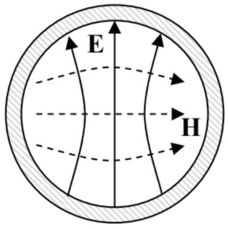Fig. 7.24. Transverse field components in the fundamental \(\ H_{11}\) mode of a metallic, circular waveguide (schematically).

One can see that the field structure is actually very similar to that of the fundamental mode in the rectangular waveguide, shown in Fig. 22, despite the different nomenclature (which is due to the different coordinates used for the solution). However, note the arbitrary constant angle \(\ \varphi_{0}\), indicating that in circular waveguides the transverse field’s polarization is arbitrary. For some practical applications, such degeneracy of these “quasi-linearly-polarized” waves creates problems; some of them may be avoided by using waves with circular polarization.

As Table 1 shows, the next lowest \(\ H\)-mode is \(\ \mathrm{H}_{21}\), for which \(\ k_{t}=k_{21}=\xi_{21}^{\prime} / R \approx 3.05 / R\), almost twice larger than that of the fundamental mode, and only then comes the first mode with no angular dependence of any field, \(\ H_{01}\), with \(\ k_{t}=k_{01}=\xi_{01}^{\prime} / R \approx 3.83 / R\),⁵⁷ followed by several angle-dependent modes: \(\ H_{31}\), \(\ H_{12}\), etc.

For the \(\ E\) modes, we may still use Eq. (141) (with \(\ f=E_{z}\)), but with the boundary condition (124) at \(\ \rho=R\). This gives the following equation for the problem eigenvalues:

\[\ J_{n}\left(k_{n m} R\right)=0, \text { i.e. } k_{n m}=\frac{\xi_{n m}}{R},\tag{7.145}\]

where \(\ \xi_{n m}\) is the \(\ m^{\text {th }}\) zero of function \(\ J_{n}(\xi)\) – see Table 2.1. The table shows that the lowest \(\ k_{t}\) is equal to \(\ \xi_{01} / R \approx 2.405 / R\). Hence the corresponding mode \(\ \left(E_{01}\right)\), with no angular dependence of its fields, e.g.

\[\ E_{z}=E_{l} J_{0}\left(\xi_{01} \frac{\rho}{R}\right),\tag{7.146}\]

has the second-lowest cutoff frequency, ~30% higher than that of the fundamental mode \(\ H_{11}\).

Finally, let us discuss one more topic of general importance – the number \(\ N\) of electromagnetic modes that may propagate in a waveguide within a certain range of relatively large frequencies \(\ \omega>>\omega_{\mathrm{c}}\). It is easy to calculate for a rectangular waveguide, with its simple expressions (132) for the eigenvalues of \(\ \left\{k_{x}, k_{y}\right\}\). Indeed, these expressions describe a rectangular mesh on the \(\ \left[k_{x}, k_{y}\right]\) plane, so that each point corresponds to the plane area \(\ \Delta A_{k}=(\pi / a)(\pi / b)\), and the number of modes in a large \(\ k\)-plane area \(\ A_k>>\Delta A_{k}\) is \(\ N=A_{k} / \Delta A_{k}=a b A_{k} / \pi^{2}=A A_{k} / \pi^{2}\), where \(\ A\) is the waveguide’s cross-section area.⁵⁸ However, it is frequently more convenient to discuss transverse wave vectors \(\ \mathbf{k}_{t}\) of arbitrary direction, i.e. with an arbitrary sign of their components \(\ k_{x}\) and \(\ k_{y}\). Taking into account that the opposite values of each component actually give the same wave, the actual number of different modes of each type (\(\ E\)- or \(\ H\)-) is a factor of \(\ 2^{2} \equiv 4\) lower than was calculated above. This means that the number of modes of both types is

\[\ N=2 \frac{A_{k} A}{(2 \pi)^{2}}.\tag{7.147}\]

Let me leave it for the reader to find hand-waving (but convincing :-) arguments that this mode counting rule is valid for waveguides with cross-sections of any shape, and any boundary conditions on the walls, provided that \(\ N >>1\).

---

Reference

⁵² For the derivation of Eqs. (121), one of two linear equations (100) should be first vector-multiplied by \(\ \mathbf{n}_{z}\). Note that this approach could not be used to analyze the TEM waves, because for them \(\ k_{t}=0, E_{z}=0, H_{z}=0\), and Eqs. (121) yield uncertainty.

⁵³ An interesting recent twist in the ideas of electromagnetic metamaterials (mentioned in Sec. 5 above) is the so-called \(\ \varepsilon\text {-near-zero }\) materials, designed to have the effective product \(\ \varepsilon \mu\) much lower than \(\ \varepsilon_{0} \mu_{0}\) within certain frequency ranges. Since at these frequencies the speed \(\ \nu\) (4) becomes much lower than \(\ c\), the cutoff frequency (123) virtually vanishes. As a result, the waves may “tunnel” through very narrow sections of metallic waveguides filled with such materials – see, e.g., M. Silveirinha and N. Engheta, Phys. Rev. Lett. 97, 157403 (2006).

⁵⁴ Let me hope that the solution of equations of the type \(\ d^{2} X / d x^{2}+k_{x}^{2} X=0\) does not present any problem for the reader, at least due to their prior experience with problems such as standing waves on a guitar string, wavefunctions in a flat 1D quantum well, or (with the replacement \(\ x \rightarrow t\)) a classical harmonic oscillator.

⁵⁵ Otherwise, the function \(\ H_{z}(x, y)\) would be constant, so that, according to Eq. (121), the transverse components of the electric and magnetic field would equal zero. As a result, as the last two lines of Eqs. (100) show, the whole field would be zero for any \(\ k_{z} \neq 0\).

⁵⁶ Mathematically, the lowest root of Eq. (142) with \(\ n = 0\) equals 0. However, it would yield \(\ k = 0\) and hence a constant field \(\ H_{z}\), which, according to the first of Eqs. (121), would give a vanishing electric field.

⁵⁷ The electric field lines in the \(\ H_{01}\) mode (as well as all higher \(\ H_{0 m}\) modes) are directed straight from the symmetry axis to the walls, reminding those of the TEM waves in the coaxial cable. Due to this property, these modes provide, at \(\ \omega>>\omega_{\mathrm{c}}\), much lower energy losses (see Sec. 9 below) than the fundamental \(\ H_{11}\) mode, and are sometimes used in practice, despite the inconvenience of working in the multimode frequency range.

⁵⁸ This formula ignores the fact that, according to the above analysis, some modes (with \(\ n = 0\) and \(\ m = 0\) for the \(\ H\) modes, and \(\ n = 0\) or \(\ m = 0\) for the \(\ E\) modes) are forbidden. However, for \(\ N >> 1\), the associated corrections of Eq. (147) are negligible.