7.10: Exercise Problems

7.1.^* Find the temporal Green’s function of a medium whose complex dielectric constant obeys the Lorentz oscillator model given by Eq. (32), using:

(i) the Fourier transform, and

(ii) the direct solution of Eq. (30).

Hint: For the Fourier-transform approach, you may like to use the Cauchy integral.⁹⁰

7.2. The electric polarization of some material responds in the following way to an electric field step:⁹¹

\[\ P(t)=\varepsilon_{1} E_{0}\left(1-e^{-t / \tau}\right), \quad \text { if } E(t)=E_{0} \times \begin{cases}0, & \text { for } t<0, \\ 1, & \text { for } 0<t,\end{cases}\]

where \(\ \tau\) is a positive constant. Calculate the complex permittivity \(\ \varepsilon(\omega)\) of this material, and discuss a possible simple physical model giving such dielectric response.

7.3. Calculate the complex dielectric constant \(\ \varepsilon(\omega)\) for a material whose dielectric-response Green’s function, defined by Eq. (23), is

\[\ G(\theta)=G_{0}\left(1-e^{-\theta / \tau}\right),\]

with some positive constants \(\ G_{0}\) and \(\ \tau\). What is the difference between this dielectric response and the apparently similar one considered in the previous problem?

7.4. Use the Lorentz oscillator model of an atom, given by Eq. (30), to calculate the average potential energy of the atom in a uniform, sinusoidal ac electric field, and use the result to calculate the potential profile created for the atom by a standing electromagnetic wave with the electric field amplitude \(\ E_{\omega}(\mathbf{r})\).

7.5. The solution of the previous problem shows that a standing, plane electromagnetic wave exerts a time-averaged force on a non-relativistic charged particle. Reveal the physics of this force by writing and solving the equations of motion of a free, charged particle in:

(i) a linearly-polarized, monochromatic, plane traveling wave, and

(ii) a similar but standing wave.

7.6. Calculate, sketch, and discuss the dispersion relation for electromagnetic waves propagating in a medium described by Eq. (32), for the case of negligible damping.

7.7. As was briefly discussed in Sec. 2,⁹² a wave pulse of a finite but relatively large spatial extension \(\ \Delta z>>\lambda \equiv 2 \pi / k\) may be formed as a wave packet – a sum of sinusoidal waves with wave vectors k within a relatively narrow interval. Consider an electromagnetic plane wave packet of this type, with the electric field distribution

\(\ \mathbf{E}(\mathbf{r}, t)=\operatorname{Re} \int_{-\infty}^{+\infty} \mathbf{E}_{k} e^{i\left(k z-\omega_{k} t\right)} d k, \quad \text { with } \omega_{k}\left[\varepsilon\left(\omega_{k}\right) \mu\left(\omega_{k}\right)\right]^{1 / 2} \equiv|k|,\)

propagating along the z-axis in an isotropic, linear, and loss-free (but not necessarily dispersion-free) medium. Express the full energy of the packet (per unit area of wave’s front) via the complex amplitudes \(\ \mathbf{E}_{k}\), and discuss its dependence on time.

7.8.^* Analyze the effect of a constant, uniform magnetic field \(\ \mathbf{B}_{0}\), parallel to the direction n of electromagnetic wave propagation, on the wave’s dispersion in plasma, within the same simple model that was used in Sec. 2 for the derivation of Eq. (38). (Limit your analysis to relatively weak waves, whose magnetic field is negligible in comparison with \(\ \mathbf{B}_{0}\).)

Hint: You may like to represent the incident wave as a linear superposition of two circularly polarized waves, with opposite polarization directions.

7.9. A monochromatic, plane electromagnetic wave is normally incident, from free space, on a uniform slab of a material with electric permittivity \(\ \varepsilon\) and magnetic permeability \(\ \mu\), with the slab thickness \(\ d\) comparable with the wavelength.

(i) Calculate the power transmission coefficient \(\ \mathcal{T}\), i.e. the fraction of the incident wave’s power, that is transmitted through the slab.

(ii) Assuming that \(\ \varepsilon\) and \(\ \mu\) are frequency-independent and positive, analyze in detail the frequency dependence of \(\ \mathcal{T}\). In particular, how does the function \(\ \mathcal{T}(\omega)\) depend on the slab’s thickness \(\ d\) and the wave impedance \(\ Z=(\mu / \varepsilon)^{1 / 2}\) of its material?

7.10. A monochromatic, plane electromagnetic wave, with free-space wave number \(\ k_{0}\), is normally incident on a plane, conducting film of thickness \(\ d \sim \delta_{\mathrm{s}}<1 / k_{0}\). Calculate the power transmission coefficient of the system, i.e. the fraction of the incident wave’s power propagating beyond the film. Analyze the result in the limits of small and large ratio \(\ d / \delta_{\mathrm{s}}\).

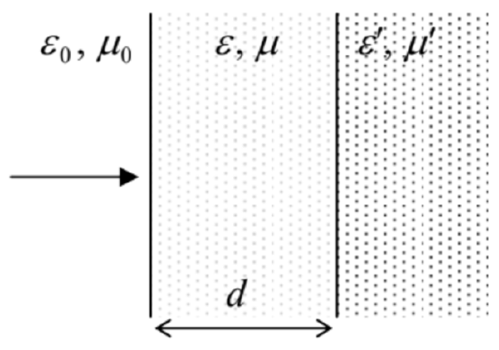
7.11. A plane wave of frequency \(\ \omega\) is normally incident, from free space, on a plane surface of a material with real electric permittivity \(\ \varepsilon^{\prime}\) and magnetic permeability \(\ \mu^{\prime}\). To minimize the wave’s reflection from the surface, you may cover it with a layer, of thickness \(\ d\), of another transparent material – see the figure on the right. Calculate the optimal values of \(\ \varepsilon\), \(\ \mu\), and \(\ d\).

7.12. A monochromatic, plane wave is incident from inside a medium with \(\ \varepsilon \mu>\varepsilon_{0} \mu_{0}\) onto its plane surface, at an angle of incidence \(\ \theta\) larger than the critical angle \(\ \theta_{\mathrm{c}}=\sin ^{-1}\left(\varepsilon_{0} \mu_{0} / \varepsilon \mu\right)^{1 / 2}\). Calculate the depth \(\ \delta\) of the evanescent wave penetration into the free space, and analyze its dependence on \(\ \theta\). Does the result depend on the wave’s polarization?

7.13. Analyze the possibility of propagation of surface electromagnetic waves along a plane boundary between plasma and free space. In particular, calculate and analyze the dispersion relation of the waves.

Hint: Assume that the magnetic field of the wave is parallel to the boundary and perpendicular to the wave’s propagation direction. (After solving the problem, justify this mode choice.)

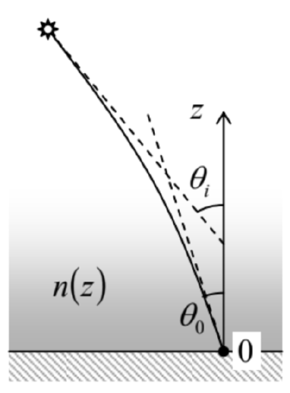
7.14. Light from a very distant source arrives to an observer through a plane layer of nonuniform medium with a certain refraction index distribution, \(\ n(z)\), at angle \(\ \theta_{0}\) – see the figure on the right. What is the genuine direction \(\ \theta_{i}\) to the source, if \(\ n(z) \rightarrow 1\) at \(\ z \rightarrow \infty\)? (This problem is evidently important for high-precision astronomical measurements from the Earth surface.)

7.15. Calculate the impedance \(\ Z_{W}\) of the long, straight TEM transmission lines formed by metallic electrodes with the cross-sections shown in the figure below:

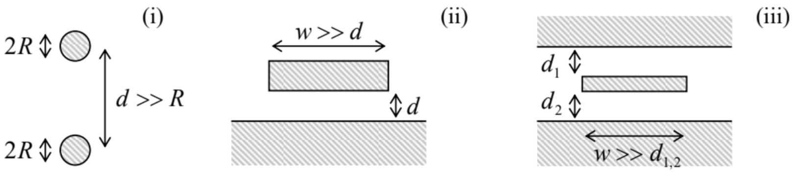
(i) two round, parallel wires separated by distance \(\ d >>R\),

(ii) a microstrip line of width \(\ w >> d\),

(iii) a stripline with \(\ w >> d_{1} \sim d_{2}\),

in all cases using the coarse-grain boundary conditions on metallic surfaces. Assume that the conductors are embedded into a linear dielectric with constant \(\ \varepsilon\) and \(\ \mu\).

7.16. Modify the solution of Task (ii) of the previous problem for a superconductor microstrip line, taking into account the magnetic field penetration into both the strip and the ground plane.

7.17.^* What lumped ac circuit would be equivalent to the TEM-line system shown in Fig. 19, with an incident wave’s power \(\ \mathscr{P}_{\mathrm{i}}\)? Assume that the wave reflected from the lumped load circuit does not return to it.

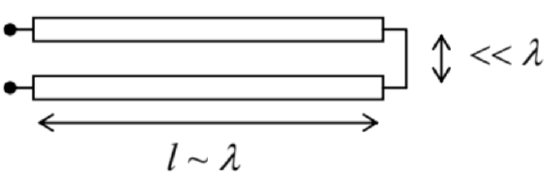
7.18. Find the lumped ac circuit equivalent to a loss-free TEM transmission line of length \(\ l \sim \lambda\), with a small cross-section area \(\ A<<\lambda^{2}\), as “seen” (measured) from one end, if the line’s conductors are galvanically connected (“shortened”) at the other end – see the figure on the right. Discuss the result’s dependence on the signal frequency.

7.19. Represent the fundamental \(\ H_{10}\) wave in a rectangular waveguide (Fig. 22) with a sum of two plane waves, and discuss the physics behind such a representation.

7.20.^* For a metallic coaxial cable with the circular cross-section (Fig. 20), find the lowest non-TEM mode and calculate its cutoff frequency.

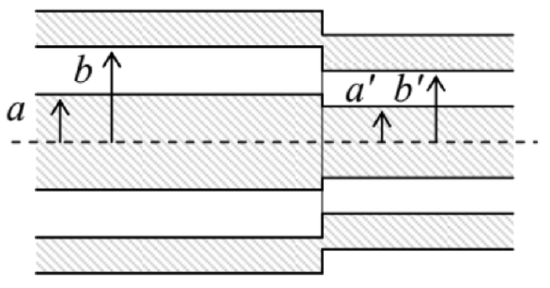
7.21. Two coaxial cable sections are connected coaxially – see the figure on the right, which shows the cut along the system’s symmetry axis. Relations (118) and (120) seem to imply that if the ratios \(\ b / a\) of these sections are equal, their impedance matching is perfect, i.e. a TEM wave incident from one side on the connection would pass it without any reflection at all: \(\ R = 0\). Is this statement correct?

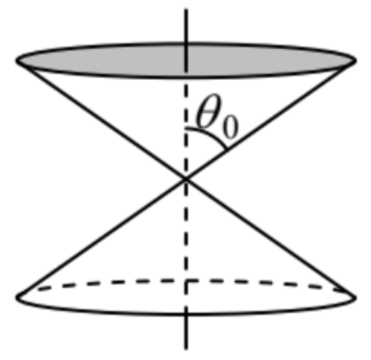
7.22. Prove that TEM-like waves may propagate, in the radial direction, in the free space between two coaxial, round, metallic cones – see the figure on the right. Can this system be characterized by a certain transmission line impedance \(\ Z_{W}\), as defined by Eq. (7.115)?

7.23.^* Use the recipe outlined in Sec. 7 to prove the characteristic equation (161) for the \(\ HE\) and \(\ EH\) modes in step-index optical fiber with a round cross-section.

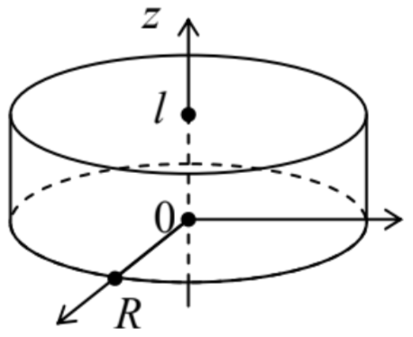
7.24. Neglecting the skin-effect depth \(\ \delta_{\mathrm{s}}\), find the lowest eigenfrequencies, and the corresponding field distributions, of standing electromagnetic waves inside a round cylindrical resonant cavity – see the figure on the right.

7.25. A plane, monochromatic wave propagates through a medium with an Ohmic conductivity \(\ \sigma\), and negligible electric and magnetic polarization effects. Calculate the wave’s attenuation, and relate the result with a certain calculation carried out in Chapter 6.

7.26. Generalize the telegrapher’s equations (110)-(111) by accounting for small energy losses:

(i) in the transmission line’s conductors, and

(ii) in the medium separating the conductors,

using their simplest (Ohmic) models. Formulate the conditions of validity of the resulting equations.

7.27. Calculate the skin-effect contribution to the attenuation coefficient \(\ \alpha\), defined by Eq. (214), for the fundamental \(\ \left(H_{10}\right)\) mode propagating in a metallic-wall waveguide with a rectangular cross-section – see Fig.22. Use the results to evaluate the wave decay length \(\ l_{\mathrm{d}} \equiv 1 / \alpha\) of a 10 GHz wave in the standard X-band waveguide WR-90 (with copper walls, \(\ a=23 \mathrm{~mm}, b=10 \mathrm{~mm}\), and no dielectric filling), at room temperature. Compare the result with that (obtained in Sec. 9) for the standard TV coaxial cable, at the same frequency.

7.28.^* Calculate the skin-effect contribution to the attenuation coefficient \(\ \alpha\) of

(i) the fundamental \(\ \left(H_{11}\right)\) wave, and

(ii) the \(\ H_{01}\) wave,

in a metallic-wall waveguide with the circular cross-section (see Fig. 23a), and analyze the low-frequency \(\ \left(\omega \rightarrow \omega_{\mathrm{c}}\right)\) and high-frequency \(\ \left(\omega>>\omega_{\mathrm{c}}\right)\) behaviors of \(\ \alpha\) for each of these modes.

7.29. For a rectangular metallic-wall resonator with dimensions \(\ a \times b \times l(b \leq a, l)\), calculate the \(\ Q\)-factor in the fundamental oscillation mode, due to the skin-effect losses in the walls. Evaluate the factor for a \(\ 23 \times 23 \times 10 \mathrm{~mm}^{3}\) resonator with copper walls, at room temperature.

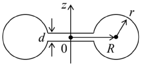
7.30.^* Calculate the lowest eigenfrequency and the \(\ Q\)-factor (due to the skin-effect losses) of the toroidal (axially-symmetric) resonator with metallic walls, and the interior cross-section shown in the figure on the right, in the case when \(\ d<<r, R\).

7.31. Express the contribution to the damping coefficient (the reciprocal \(\ Q\)-factor) of a resonator, from small energy losses in the dielectric that fills it, via the complex functions \(\ \varepsilon(\omega)\) and \(\ \mu(\omega)\) of the material.

7.32. For the dielectric Fabry-Pérot resonator (Fig. 31) with the normal wave incidence, calculate the \(\ Q\)-factor due to radiation losses, in the limit of a strong impedance mismatch \(\ \left(Z>>Z_{0}\right)\), using two approaches:

(i) from the energy balance, using Eq. (227), and

(ii) from the frequency dependence of the power transmission coefficient, using Eq. (229).

Compare the results.

---

Reference

⁹⁰ See, e.g., MA Eq. (15.2).

⁹¹ This function E(t) is of course proportional to the well-known step function \(\ \theta(t)\) – see, e.g., MA Eq. (14.3). I am not using this notion just to avoid possible confusion between two different uses of the Greek letter \(\ \theta\).

⁹² And in more detail in CM Sec. 5.3, and especially in QM Sec. 2.2.