
2.9: Periodic Systems- Particle Dynamics


- Last updated
- Jan 29, 2022
- Save as PDF

( \newcommand{\kernel}{\mathrm{null}\,}\)
The band structure of the energy spectrum of a particle moving in a periodic potential has profound implications not only for its density of states but also for its dynamics. Indeed, let us consider the simplest case of a wave packet composed of the Bloch functions (210), all belonging to the same (say, nth ) energy band. Similarly to Eq. (27) for a free particle, we can describe such a packet as Ψ(x,t)=∫aquq(x)ei[qx−ω(q)t]dq, where the a-periodic functions u(x), defined by Eq. (208), are now indexed to emphasize their dependence on the quasimomentum, and ω(q)≡En(q)/ℏ is the function of q describing the shape of the corresponding energy band - see, e.g., Fig. 26b or Fig. 28. If the packet is narrow in the q-space, i.e. if the width δq of the distribution aq is much smaller than all the characteristic q-scales of the dispersion relation ω(q), in particular of π/a, we may simplify Eq. (234) exactly as it was done in Sec. 2 for a free particle, despite the presence of the periodic factors uq(x) under the integral. In the linear approximation of the Taylor expansion, we get a full analog of Eq. (32), but now with q rather than k, and vgr=dωdq∣q=q0, and vph=ωq∣q=q0, where q0 is the central point of the quasimomentum distribution. Despite the formal similarity with Eqs. (33) for the free particle, this result is much more eventful. For example, as evident from the dispersion relation’s topology (see Figs. 26b, 28), the group velocity vanishes not only at q=0, but at all values of q that are multiples of (π/a), at the bottom and on the top of each energy band. Even more intriguing is that the group velocity’s sign changes periodically with q.
This group velocity alternation leads to fascinating, counter-intuitive phenomena if a particle placed in a periodic potential is the subject of an additional external force F(t). (For electrons in a crystal, this may be, for example, the force of the applied electric field.) Let the force be relatively weak, so that the product Fa (i.e. the scale of the energy increment from the additional force per one lattice period) is much smaller than both relevant energy scales of the dispersion relation E(q)− see Fig. 26b: Fa<<ΔEn,Δn. This strong relationship allows one to neglect the force-induced interband transitions, so that the wave packet (234) includes the Bloch eigenfunctions belonging to only one (initial) energy band at all times. For the time evolution of its center q0, theory yields 68 an extremely simple equation of motion ˙q0=1ℏF(t). This equation is physically very transparent: it is essentially the 2nd Newton law for the time evolution of the quasimomentum ℏq under the effect of the additional force F(t) only, excluding the periodic force −∂U(x)/∂x of the background potential U(x). This is very natural, because as Eq. (210) implies, ℏq is essentially the particle’s momentum averaged over the potential’s period, and the periodic force effect drops out at such an averaging.
Despite the simplicity of Eq. (237), the results of its solution may be highly nontrivial. First, let us use Eqs. (235) and (237) to find the instant group acceleration of the particle (i.e. the acceleration of its wave packet’s envelope): agr≡dvgrdt≡ddtdω(q0)dq0≡ddq0dω(q0)dq0dq0dt=d2ω(q0)dq20dq0dt=1ℏd2ωdq2|q=q0F(t). This means that the second derivative of the dispersion ω(q) relation (specific for each energy band) plays the role of the effective reciprocal mass of the particle at this particular value of q0 : mef=ℏd2ω/dq2≡ℏ2d2En/dq2. For the particular case of a free particle, for which Eq. (216) is exact, this expression is reduced to the original (and constant) mass m, but generally, the effective mass depends on the wave packet’s momentum. According to Eq. (239), at the bottom of any energy band, mef is always positive but depends on the strength of the particle’s interaction with the periodic potential. In particular, according to Eq. (206), in the tight-binding limit, the effective mass is very large: |mef|q=(π/a)n=ℏ22δna2≡mE(1)π2δn≫m. On the contrary, in the weak-potential limit, the effective mass is close to m at most points of each energy band, but at the edges of the (narrow) bandgaps, it is much smaller. Indeed, expanding Eq. (224) in the Taylor series near point q=qm, we get E±|E≈E(n)−Eave≈±|Un|±12|Un|(dEldq)2q=qm˜q2=±|Un|±γ22|Un|˜q2, where γ and ˜q are defined by Eq. (225), so that |mef|q=qm=|Un|ℏ2γ2≡m|Un|2E(n)<<m. The effective mass effects in real atomic crystals may be very significant. For example, the charge carriers in silicon have mef≈0.19me in the lowest, normally-empty energy band (traditionally called the conduction band), and mef≈0.98me in the adjacent lower, normally-filled valence band. In some semiconducting compounds, the conduction-band mass may be even smaller - down to 0.0145 me in InSb!
However, the effective mass’ magnitude is not the most surprising effect. A more fascinating corollary of Eq. (239) is that on the top of each energy band the effective mass is negative - please revisit Figs. 26b, 28, and 29 again. This means that the particle (or more strictly, its wave packet’s envelope) is accelerated in the direction opposite to the applied force. This is exactly what electronic engineers, working with electrons in semiconductors, call holes, characterizing them by a positive mass |mef |, but compensating this sign change by taking their charge e positive. If the particle stays in close vicinity of the energy band’s top (say, due to frequent scattering effects, typical for the semiconductors used in engineering practice), such double sign flip does not lead to an error in calculations of hole’s dynamics, because the electric field’s force is proportional to the particle’s charge, so that the particle’s acceleration agr is proportional to the charge-to-mass ratio. 69
However, in some phenomena such simple representation is unacceptable. 70 For example, let us form a narrow wave packet at the bottom of the lowest energy band, 71 and then exert on it a constant force F>0 - say, due to a constant external electric field directed along the x-axis. According to Eq. (237), this force would lead to linear growth of q0 in time, so that in the quasimomentum space, the packet’s center would slide, with a constant speed, along the q axis - see Fig. 33a. Close to the energy band’s bottom, this motion would correspond to a positive effective mass (possibly, somewhat different than the genuine particle’s mass m ), and hence be close to the free particle’s acceleration. However, as soon as q0 has reached the inflection point where d2E1/dq2=0, the effective mass, and hence its acceleration (238) change signs to negative, i.e. the packet starts to slow down (in the direct space), while still moving ahead with the same velocity in the quasimomentum space. Finally, at the energy band’s top, the particle stops at a certain xmax, while continuing to move forward in the q-space.
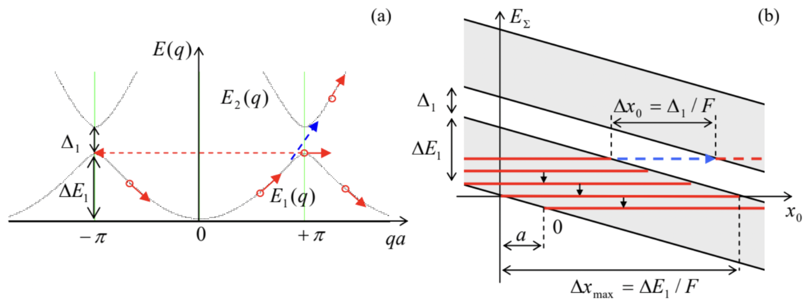
Now we have two alternative ways to look at the further time evolution of the wave packet along the quasimomentum’s axis. From the extended zone picture (which is the simplest for this analysis, see Fig. 33a), 72 we may say that the particle crosses the 1st Brillouin zone boundary and continues to go forward in q-space, i.e. down the lowest energy band. According to Eq. (235), this region (up to the next energy minimum at qa=2π ) corresponds to a negative group velocity. After q0 has reached that minimum, the whole process repeats again - and again, and again.
These are the famous Bloch oscillations - the effect which had been predicted, by the same F. Bloch, as early as 1929 but evaded experimental observation until the 1980s (see below) due to the strong scattering effects in real solid-state crystals. The time period of the oscillations may be readily found from Eq. (237): ΔtB=Δqdq/dt=2π/aF/ℏ=2πℏFa, so that their frequency may be expressed by a very simple formula
ωB≡2πΔtB=Faℏ, and hence is independent of any peculiarities of the energy band/gap structure.
The direct-space motion of the wave packet’s center x0(t) during the Bloch oscillation process may be analyzed by integrating the first of Eqs. (235) over some time interval Δt, and using Eq. (237): Δx0(t)≡∫Δt0vgrdt=∫Δt0dω(q0)dq0dt≡∫Δt0dω(q0)dq0/dt=ℏF∫t=Δtt=0dω=ℏFΔω(q0). If the interval Δt is equal to the Bloch oscillation period ΔtB(243), the initial and final values of E(q0)= ℏω(q0) are equal, giving Δx0=0 : in the end of the period, the wave packet returns to its initial position in space. However, if we carry out this integration only from the smallest to the largest values of ω(q0), i.e. the adjacent points where the group velocity vanishes, we get the following Bloch oscillation swing: Δxmax=ℏF(ωmax−ωmin)≡ΔE1F. This simple result may be interpreted using an alternative energy diagram (Fig. 33b), which results from the following arguments. The additional force F may be described not only via the 2nd Newton law’s version (237), but, alternatively, by its contribution −Fx to the Gibbs potential energy 73 UΣ(x)=U(x)−Fx The exact solution of the Schrödinger equation (61) with such a potential may be hard to find directly, but if the force F is sufficiently weak, as we are assuming throughout this discussion, the second term in Eq. (247) may be considered as a constant on the scale of a<<Δxmax. In this case, our quantummechanical treatment of the periodic potential U(x) is still virtually correct, but with an energy shift depending on the "global" position x0 of the packet’s center. In this approximation, the total energy of the wave packet is EΣ=E(q0)−Fx0. In a plot of such energy as a function of x0 (Fig. 33b), the energy dependence on q0 is hidden, but as was discussed above, it is rather uneventful and may be well characterized by the position of bandgap edges on the energy axis. 74 In this representation, the Bloch oscillations keep the full energy EΣ of the particle constant, i.e. follow a horizontal line in Fig. 33b, limited by the classical turning points corresponding to the bottom and the top of the allowed energy band. The distance Δxmax between these points is evidently given by Eq. (246).
Besides this alternative look at the Bloch oscillation swing, the total energy diagram shown in Fig. 33b enables one more remarkable result. Let a wave packet be so narrow in the momentum space that δx∼1/δq≫Δxmax; then it may be well represented by definite energy, i.e. by a horizontal line in Fig. 33b. But Eq. (247) is exactly invariant with respect to the following simultaneous translation of the coordinate and the energy: x→x+a,E→E−Fa This means that it is satisfied by an infinite set of similar solutions, each corresponding to one of the horizontal red lines shown in Fig. 33b. This is the famous Wannier-Stark ladder 75 with the step height ΔEwS=Fa. The importance of this alternative representation of the Bloch oscillations is due to the following fact. In most experimental realizations, the power of the electromagnetic radiation with frequency (244), that may be extracted from the oscillations of a charged particle, is very low, so that their direct detection represents a hard problem. 76 However, let us apply to a Bloch oscillator an additional ac field at frequency ω≈ωB. As these frequencies are brought close together, the external signal should synchronize ("phase-lock") the Bloch oscillations, 77 resulting in certain changes of time-independent observables - for example, a resonant change of absorption of the external radiation. Now let us notice that the combination of Eqs. (244) and (250) yield the following simple relation: ΔEwS=ℏωB. This means that the phase-locking at ω≈ωB allows for an alternative (but equivalent) interpretation − as the result of ac-field-induced quantum transitions 78 between the steps of the Wannier-Stark ladder. (Again, such occasions when two very different languages may be used for alternative interpretations of the same effect is one of the most beautiful features of physics.)
This phase-locking effect has been used for the first experimental confirmations of the Bloch oscillation theory. 79 For this purpose, the natural periodic structures, solid-state crystals, are inconvenient due to their very small period a∼10−10 m. Indeed, according to Eq. (244), such structures require very high forces F (and hence very high electric fields E=F/e ) to bring ωB to an experimentally convenient range. This problem has been overcome using artificial periodic structures (superlattices) of certain semiconductor compounds, such as Ga1−xAlxAs with various degrees x of the gallium-toaluminum atom replacement, whose layers may be grown over each other epitaxially, i.e., with very few crystal structure violations. Such superlattices, with periods a∼10 nm, have enabled a clear observation of the resonance at ω≈ωB, and hence a measurement of the Bloch oscillation frequency, in particular its proportionality to the applied dc electric field, predicted by Eq. (244).
Very soon after this discovery, the Bloch oscillations were observed 80 in small Josephson junctions, where they result from the quantum dynamics of the Josephson phase difference φ in a 2π periodic potential profile, created by the junction. A straightforward translation of Eq. (244) to this case (left for the reader’s exercise) shows that the frequency of such Bloch oscillations is ωB=πˉI2e, i.e. fB≡ωB2π=ˉI2e, where ˉI is the dc current passed through the junction - the effect not to be confused with the "classical" Josephson oscillations with frequency (1.75). It is curious that Eq. (252) may be legitimately interpreted as a result of a periodic transfer, through the Josephson junction, of discrete Cooper pairs (of charge 2e ), between two coherent Bose-Einstein condensates in the superconducting electrodes of the junction. 81
Next, our discussion of the Bloch oscillations was based on the premise that the wave packet of the particle stays within one (say, the lowest) energy band. However, just one look at Fig. 28 shows that this assumption becomes unrealistic if the energy gap separating this band from the next one becomes very small, Δ1→0. Indeed, in the weak-potential approximation, which is adequate in this limit, |U1| →0, the two dispersion curve branches (216) cross without any interaction, so that if our particle (meaning its the wave packet) is driven to approach that point, it should continue to move up in energy see the dashed blue arrow in Fig. 33a. Similarly, in the real-space representation shown in Fig. 33b, it is intuitively clear that at Δ1→0, the particle residing at one of the steps of the Wannier-Stark ladder should be able to somehow overcome the vanishing spatial gap Δx0=Δ1/F and to "leak" into the next band − see the horizontal dashed blue arrow on that panel.
This process, called the Landau-Zener (or "interband", or "band-to-band") tunneling, 82 is indeed possible. To analyze it, let us first take F=0, and consider what happens if a quantum particle, described by an x-long (i.e. E-narrow) wave packet, is incident from free space upon a periodic structure of a large but finite length l=Na>>a - see, e.g., Fig. 22. If the packet’s energy E is within one of the energy bands, it may evidently propagate through the structure (though may be partly reflected from its ends). The corresponding quasimomentum may be found by solving the dispersion relation for q; for example, in the weak-potential limit, Eq. (224) (which is valid near the gap) yields q=qm+˜q, with ˜q=±1γ[˜E2−|Un|2]1/2, for |Un|2≤˜E2, where ˜E≡E±−E(n) and γ=2aE(n)/πn− see the second of Eqs. (225).
Now, if the energy E is inside one of the energy gaps Δn, the wave packet’s propagation in an infinite periodic lattice is impossible, so that it is completely reflected from it. However, our analysis of the potential step problem in Sec. 3 implies that the packet’s wavefunction should still have an exponential tail protruding into the structure and decaying on some length δ - see Eq. (58) and Fig. 2.4. Indeed, a straightforward review of the calculations leading to Eq. (253) shows that it remains valid for energies within the gap as well, if the quasimomentum is understood as a purely imaginary number: ˜q→±iκ, where κ≡1γ[|Un|2−˜E2]1/2, for ˜E2≤|Un|2. With this replacement, the Bloch solution (193b) indeed describes an exponential decay of the wavefunction at length δ∼1/κ.
Returning to the effects of weak force F, in the real-space approach described by Eq. (248) and illustrated in Fig. 33b, we may recast Eq. (254) as κ→κ(x)=1γ[|Un|2−(F˜x)2]1/2 where ˜x is the particle’s (i.e. its wave packet center’s) deviation from the mid-gap point. Thus the gap creates a potential barrier of a finite width Δx0=2|Un|/F, through which the wave packet may tunnel with a non-zero probability. As we already know, in the WKB approximation (in our case requiring κΔx0>>1) this probability is just the potential barrier’s transparency T, which may be calculated from Eq. (117): −lnT=2∫κ(x)2>0κ(x)dx=2γ∫xc−xc[|Un|2−(F˜x)2]1/2d˜x=2|Un|γ2xc∫10(1−ξ2)1/2dξ. where ±xc≡±Δx0/2=±Un∣/F are the classical turning points. Working out this simple integral (or just noticing that it is a quarter of the unit circle’s area, and hence is equal to π/4), we get Landau-Zener tunneling probabilityT=exp{−π|Un|2γF}.
This famous result may be also obtained in a more complex way, whose advantage is a constructive proof that Eq. (257) is valid for an arbitrary relation between γF and |Un|2, i.e. arbitrary T, while our simple derivation was limited to the WKB approximation, valid only at T<<1.83 Using Eq. (225), we may rewrite the product γF participating in Eq. (257), as
where u has the meaning of the "speed" of the energy level crossing in the absence of the gap. Hence, Eq. (257) may be rewritten in the form T=exp{−2π|Un|2ℏu} which is more transparent physically. Indeed, the fraction 2|Un|/u=Δnu gives the time scale Δt of the energy’s crossing the gap region, and according to the Fourier transform, its reciprocal, ωmax∼1/Δt gives the upper cutoff of the frequencies essentially involved in the Bloch oscillation process. Hence Eq. (259) means that −lnT≈Δnℏωmax. This formula allows us to interpret the Landau-Zener tunneling as the system’s excitation across the energy gap Δn by the highest-energy quantum ℏωmax available from the Bloch oscillation process. This interpretation remains valid even in the opposite, tight-binding limit, in which, according to Eqs. (206) and (237), the Bloch oscillations are purely sinusoidal, so that the Landau-Zener tunneling is completely suppressed at ℏωB<Δ1.
Interband tunneling is an important ingredient of several physical phenomena and even some practical electron devices, for example, the tunneling (or "Esaki") diodes. This simple device is just a junction of two semiconductor electrodes, one of them so strongly n-doped by electron donors that some electrons form a degenerate Fermi gas at the bottom of the conduction band. 84 Similarly, the counterpart semiconductor electrode is p-doped so strongly that the Fermi level in the valence band is shifted below the band edge − see Fig. 34.
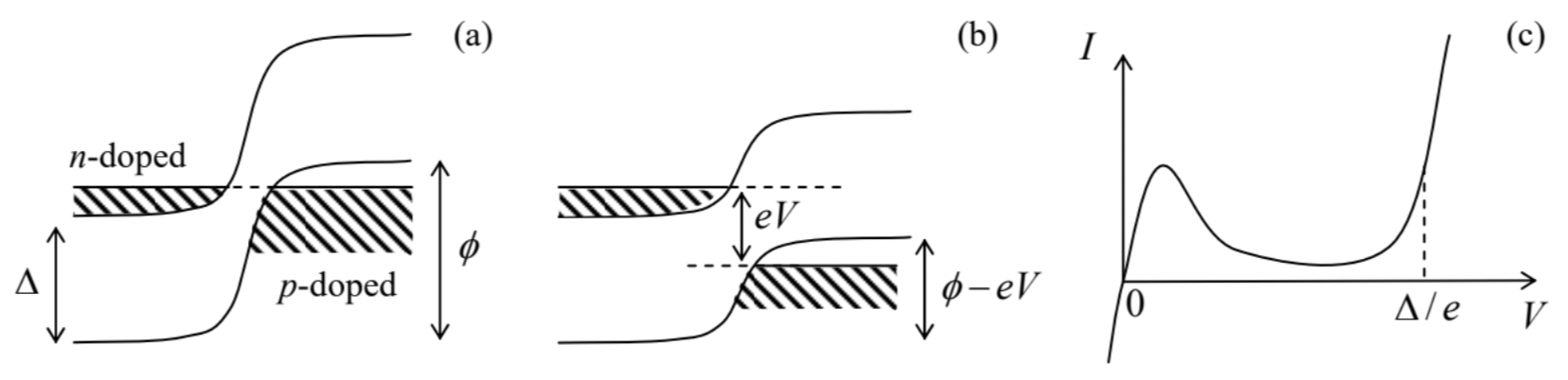
In thermal equilibrium, and in the absence of external voltage bias, the Fermi levels of the two electrodes self-align, leading to the build-up of the contact potential difference \phile, with ϕ a bit larger than the energy bandgap Δ - see Fig. 34a. This potential difference creates an internal electric field that tilts the energy bands (just as the external field did in Fig. 33b), and leads to the formation of the socalled depletion layer, in which the Fermi level is located within the energy gap and hence there are no charge carriers ready to move. In the usual p−n junctions, this layer is broad and prevents any current at applied voltages V lower than ∼Δ/e. In contrast, in a tunneling diode the depletion layer is so thin (below ∼10 nm ) that the interband tunneling is possible and provides a substantial Ohmic current at small applied voltages − see Fig. 34c. However, at larger positive biases, with eV∼Δ/2, the conduction band is aligned with the middle of the energy gap in the p-doped electrode, and electrons cannot tunnel there. Similarly, there are no electrons in the n-doped semiconductor to tunnel into the available states just above the Fermi level in the p-doped electrode - see Fig. 34b. As a result, at such voltages the current drops significantly, to grow again only when eV exceeds ∼Δ, enabling electron motion within each energy band. Thus the tunnel junction’s I−V curve has a part with a negative differential resistance (dV/dI<0) - see Fig. 34c. This phenomenon, equivalent in its effect to negative kinematic friction in mechanics, may be used for amplification of weak analog signals, for self-excitation of electronic oscillators 85 (i.e. an ac signal generation), and for signal swing restoration in digital electronics.
68 The proof of Eq. (237) is not difficult, but becomes more compact in the bra-ket formalism, to be discussed in Chapter 4. This is why I recommend to the reader its proof as an exercise after reading that chapter. For a generalization of this theory to the case of essential interband transitions see, e.g., Sec. 55 in E. Lifshitz and L. Pitaevskii, Statistical Physics, Part 2, Pergamon, 1980.
69 More discussion of this issue may be found in SM Sec. 6.4.
70 The balance of this section describes effects that are not discussed in most quantum mechanics textbooks. Though, in my opinion, every educated physicist should be aware of them, some readers may skip them at the first reading, jumping directly to the next Sec. 9 .
71 Physical intuition tells us (and the theory of open systems, to be discussed in Chapter 7, confirms) that this may be readily done, for example, by weakly coupling the system to a relatively low-temperature environment, and letting it relax to the lowest possible energy.
72 This phenomenon may be also discussed from the point of view of the reduced zone picture, but then it requires the introduction of instant jumps between the Brillouin zone boundary points (see the dashed red line in Fig. 33) that correspond to physically equivalent states of the particle. Evidently, for the description of this particular phenomenon, this language is more artificial.
73 Physically, this is just the relevant part of the potential energy of the total system comprised of our particle (in the periodic potential) and the source of the force F− see, e.g., CM Sec. 1.4.
74 In semiconductor physics and engineering, such spatial band-edge diagrams are virtually unavoidable components of almost every discussion/publication. In this series, a few more examples of such diagrams may be found in SM Sec. 6.4.
75 This effect was first discussed in detail by Gregory Hugh Wannier in his 1959 monograph on solid-state physics, while the name of Johannes Stark is traditionally associated with virtually any electric field effect on atomic systems, after he had discovered the first of such effects in 1913.
76 In systems with many independent particles (such as electrons in semiconductors), the detection problem is exacerbated by the phase incoherence of the Bloch oscillations performed by each particle. This drawback is absent in atomic Bose-Einstein condensates whose Bloch oscillations (in a periodic potential created by standing optical waves) were eventually observed by M. Ben Dahan et al., Phys. Rev. Lett. 76,4508 (1996).
77 A simple analysis of phase locking of a classical oscillator may be found, e.g., in CM Sec. 5.4. (See also the brief discussion of the phase locking of the Josephson oscillations at the end of Sec. 1.6 of this course.)
78 A quantitative theory of such transitions will be discussed in Sec. 6.6 and then in Chapter 7.
79 E. Mendez et al., Phys. Lev. Lett. 60,2426 (1988).
80 D. Haviland et al., Z. Phys. B 85,339 (1991).
81 See, e.g., D. Averin et al., Sov. Phys. -JETP 61, 407 (1985). This effect is qualitatively similar to the transfer of single electrons, with a similar frequency f=I/e, in tunnel junctions between normal (non-superconducting) metals - see, e.g., EM Sec. 2.9 and references therein.
82 It was predicted independently by L. Landau, C. Zener, E. Stueckelberg, and E. Majorana in 1932.
83 In Chapter 6 below, Eq. (257) will be derived using a different method, based on the so-called Golden Rule of quantum mechanics, but also in the weak-potential limit, i.e. for hyperbolic dispersion law (253).
84 Here I have to rely on the reader’s background knowledge of basic semiconductor physics; it will be discussed in more detail in SM Sec. 6.4.