6.1: Time-independent Perturbations

Unfortunately, only a few problems of quantum mechanics may be solved exactly in an analytical form. Actually, in the previous chapters we have solved a substantial part of such problems for a single particle, while for multiparticle systems, the exactly solvable cases are even more rare. However, most practical problems of physics feature a certain small parameter, and this smallness may be exploited by various approximate analytical methods giving asymptotically correct results \(-\) i.e. the results whose error tends to zero at the reduction of the small parameter(s). Earlier in the course, we have explored one of them, the WKB approximation, which is adequate for a particle moving through a soft potential profile. In this chapter, we will discuss other techniques that are more suitable for other cases. The historic name for these techniques is the perturbation theory, though it is more fair to speak about several perturbative approaches, because they are substantially different for different situations.

The simplest version of the perturbation theory addresses the problem of stationary states and energy levels of systems described by time-independent Hamiltonians of the type \[\hat{H}=\hat{H}^{(0)}+\hat{H}^{(1)},\] where the operator \(\hat{H}^{(1)}\), describing the system’s "perturbation", is relatively small - in the sense that its addition to the unperturbed operator \(\hat{H}^{(0)}\) results in a relatively small change of the eigenenergies \(E_{n}\) of the system, and the corresponding eigenstates. A typical problem of this type is the 1D weakly anharmonic oscillator (Fig. 1), described by the Hamiltonian (1) with

\[\ \text{Weakly anharmonic oscillator}\quad\quad\quad\quad\hat{H}^{(0)}=\frac{\hat{p}^{2}}{2 m}+\frac{m \omega_{0}^{2} \hat{x}^{2}}{2}, \quad \hat{H}^{(1)}=\alpha \hat{x}^{3}+\beta \hat{x}^{4}+\ldots\]

with sufficiently small coefficients \(\alpha, \beta, \ldots\).

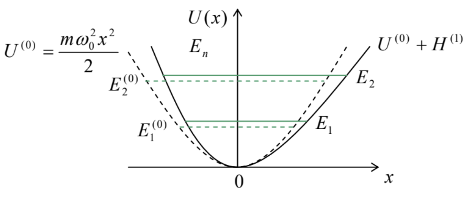Fig. 6.1. The simplest application of the perturbation theory: a weakly anharmonic 1D oscillator. (Dashed lines characterize the unperturbed, harmonic oscillator.)

I will use this system as our first example, but let me start by describing the perturbative approach to the general time-independent Hamiltonian (1). In the bra-ket formalism, the eigenproblem (4.68) for the perturbed Hamiltonian, i.e. the stationary Schrödinger equation of the system, is \[\left(\hat{H}^{(0)}+\hat{H}^{(1)}\right)|n\rangle=E_{n}|n\rangle \text {. }\] Let the eigenstates and eigenvalues of the unperturbed Hamiltonian, which satisfy the equation \[\hat{H}^{(0)}\left|n^{(0)}\right\rangle=E_{n}^{(0)}\left|n^{(0)}\right\rangle,\] be considered as known. In this case, the solution of problem (3) means finding, first, its perturbed eigenvalues \(E_{n}\) and, second, the coefficients \(\left\langle n^{,(0)} \mid n\right\rangle\) of the expansion of the perturbed state’s vectors \(|n\rangle\) in the following series over the unperturbed ones, \(\left|n^{\prime}{ }^{(0)}\right\rangle\) : \[|n\rangle=\sum_{n^{\prime}}\left|n^{\prime(0)}\right\rangle\left\langle n^{\prime(0)} \mid n\right\rangle .\] Let us plug Eq. (5), with the summation index \(n\) ’ replaced with \(n\) " (just to have a more compact notation in our forthcoming result), into both sides of Eq. (3): \[\sum_{n^{\prime \prime}}\left\langle n^{\prime \prime(0)} \mid n\right\rangle \hat{H}^{(0)}\left|n^{\prime \prime(0)}\right\rangle+\sum_{n^{\prime \prime}}\left\langle n^{\prime \prime(0)} \mid n\right\rangle \hat{H}^{(1)}\left|n^{\prime \prime(0)}\right\rangle=\sum_{n^{\prime \prime}}\left\langle n^{\prime \prime(0)} \mid n\right\rangle E_{n}\left|n^{\prime \prime(0)}\right\rangle .\] and then inner-multiply all terms by an arbitrary unperturbed bra-vector \(\left\langle n^{\prime}{ }^{(0)}\right|\) of the system. Assuming that the unperturbed eigenstates are orthonormal, \(\left\langle n^{\prime}{ }^{(0)} \mid n^{\prime,(0)}\right\rangle=\delta_{n^{\prime} n^{\prime \prime}}\), and using Eq. (4) in the first term on the left-hand side, we get the following system of linear equations \[\sum_{n^{\prime \prime}}\left\langle n^{\prime \prime(0)} \mid n\right\rangle H_{n^{\prime} n^{\prime \prime}}^{(1)}=\left\langle n^{(0)} \mid n\right\rangle\left(E_{n}-E_{n^{\prime}}^{(0)}\right),\] where the matrix elements of the perturbation are calculated, by definition, in the unperturbed brackets: \[H_{n^{\prime} n^{\prime \prime}}^{(1)} \equiv\left\langle n^{\prime(0)}\left|\hat{H}^{(1)}\right| n^{\prime \prime(0)}\right\rangle .\] The linear equation system \((7)\) is still exact, \({ }^{1}\) and is frequently used for numerical calculations. (Since the matrix coefficients (8) typically decrease when \(n\) ’ and/or \(n\) "’ become sufficiently large, the sum on the left-hand side of Eq. (7) may usually be truncated, still giving an acceptable accuracy of the solution.) To get analytical results, we need to make approximations. In the simple perturbation theory we are discussing now, this is achieved by the expansion of both the eigenenergies and the expansion coefficients into the Taylor series in a certain small parameter \(\mu\) of the problem: \[\begin{gathered} E_{n}=E_{n}^{(0)}+E_{n}^{(1)}+E_{n}^{(2)} \cdots, \\ \left\langle n^{\prime(0)} \mid n\right\rangle=\left\langle n^{\prime(0)} \mid n\right\rangle^{(0)}+\left\langle n^{(0)} \mid n\right\rangle^{(1)}+\left\langle n^{\prime \prime(0)} \mid n\right\rangle^{(2)} \cdots, \end{gathered}\] where

\[E_{n}^{(k)} \propto\left\langle n^{\prime(0)} \mid n\right\rangle^{(k)} \propto \mu^{k} .\] In order to explore the \(1^{\text {st }}\)-order approximation, which ignores all terms \(O\left(\mu^{2}\right)\) and higher, let us plug only the two first terms of the expansions (9) and (10) into the basic equation (7): \[\sum_{n^{\prime \prime}} H_{n^{n} n^{\prime \prime}}^{(1)}\left(\delta_{n^{\prime \prime} n}+\left\langle n^{\prime \prime(0)} \mid n\right\rangle^{(1)}\right)=\left(\delta_{n^{\prime} n}+\left\langle n^{\prime(0)} \mid n\right\rangle^{(1)}\right)\left(E_{n}^{(0)}+E_{n}^{(1)}-E_{n^{\prime}}^{(0)}\right) .\] Now let us open the parentheses, and disregard all the remaining terms \(O\left(\mu^{2}\right)\). The result is \[H_{n^{\prime} n}^{(1)}=\delta_{n^{\prime} n} E_{n}^{(1)}+\left\langle n^{(0)} \mid n\right\rangle^{(1)}\left(E_{n}^{(0)}-E_{n^{\prime}}^{(0)}\right),\] This relation is valid for any set of indices \(n\) and \(n\) ’; let us start from the case \(n=n\), immediately getting a very simple (and practically, the most important!) result: \[E_{n}^{(1)}=H_{n n}^{(1)} \equiv\left\langle n^{(0)}\left|\hat{H}^{(1)}\right| n^{(0)}\right\rangle\] For example, let us see what this result gives for two first perturbation terms in the weakly anharmonic oscillator (2): \[E_{n}^{(1)}=\alpha\left\langle n^{(0)}\left|\hat{x}^{3}\right| n^{(0)}\right\rangle+\beta\left\langle n^{(0)}\left|\hat{x}^{4}\right| n^{(0)}\right\rangle .\] As the reader knows (or should know :-) from the solution of Problem 5.9, the first bracket equals zero, while the second one yields \({ }^{2}\) \[E_{n}^{(1)}=\frac{3}{4} \beta x_{0}^{4}\left(2 n^{2}+2 n+1\right) .\] Naturally, there should be some non-vanishing contribution to the energies from the (typically, larger) perturbation proportional to \(\alpha\), so that for its calculation we need to explore the \(2^{\text {nd }}\) order of the theory. However, before doing that, let us complete our discussion of its \(1^{\text {st }}\) order.

For \(n^{\prime} \neq n\), Eq. (13) may be used to calculate the eigenstates rather than the eigenvalues: \[\left\langle n^{\prime(0)} \mid n\right\rangle^{(1)}=\frac{H_{n^{n} n}^{(1)}}{E_{n}^{(0)}-E_{n^{\prime}}^{(0)}}, \quad \text { for } n^{\prime} \neq n .\] This means that the eigenket’s expansion (5), in the \(1^{\text {st }}\) order, may be represented as \[\left|n^{(1)}\right\rangle=C\left|n^{(0)}\right\rangle+\sum_{n^{\prime} \neq n} \frac{H_{n^{\prime} n}^{(1)}}{E_{n}^{(0)}-E_{n^{\prime}}^{(0)}}\left|n^{(0)}\right\rangle .\] The coefficient \(C \equiv\left\langle n^{(0)} \mid n^{(1)}\right\rangle\) cannot be found from Eq. (17); however, requiring the final state \(n\) to be normalized, we see that other terms may provide only corrections \(O\left(\mu^{2}\right)\), so that in the \(1^{\text {st }}\) order we should take \(C=1\). The most important feature of Eq. (18) is its denominators: the closer are the unperturbed eigenenergies of two states, the larger is their mutual "interaction" due to the perturbation.

This feature also affects the \(1^{\text {st }}\)-order’s validity condition, which may be quantified using Eq. (17): the magnitudes of the brackets it describes have to be much less than the unperturbed bracket \(\langle n \mid n\rangle^{(0)}=1\), so that all elements of the perturbation matrix have to be much less than difference between the corresponding unperturbed energies. For the anharmonic oscillator’s energy corrections (16), this requirement is reduced to \(E_{n}{ }^{(1)}<<\hbar \omega_{0}\).

Now we are ready for going after the \(2^{\text {nd }}\)-order approximation to Eq. (7). Let us focus on the case \(n^{\prime}=n\), because as we already know, only this term will give us a correction to the eigenenergies. Moreover, since the left-hand side of Eq. (7) already has a small factor \(H_{n^{\prime} n^{\prime \prime}}^{(1)} \propto\), the bracket coefficients in that part may be taken from the \(1^{\text {st }}\)-order result (17). As a result, we get \[E_{n}^{(2)}=\sum_{n^{n}}\left\langle n^{\prime \prime(0)} \mid n\right\rangle^{(1)} H_{n n^{\prime \prime}}^{(1)}=\sum_{n^{n} \neq n} \frac{H_{n^{\prime \prime} n}^{(1)} H_{n n^{n}}^{(1)}-E_{n^{\prime \prime}}^{(0)}}{E} .\] Since \(\hat{H}^{(1)}\) has to be Hermitian, we may rewrite this expression as \[E_{n}^{(2)}=\sum_{n^{\prime} \neq n} \frac{\left|H_{n^{\prime} n}^{(1)}\right|^{2}}{E_{n}^{(0)}-E_{n^{\prime}}^{(0)}} \equiv \sum_{n^{\prime} \neq n} \frac{\left|\left\langle n^{(0)}\left|\hat{H}^{(1)}\right| n^{(0)}\right\rangle\right|^{2}}{E_{n}^{(0)}-E_{n^{\prime}}^{(0)}} .\] This is the much-celebrated \(2^{\text {nd }}\)-order perturbation result, which frequently (in sufficiently symmetric problems) is the first non-vanishing correction to the state energy - for example, from the cubic term (proportional to \(\alpha\) ) in our weakly anharmonic oscillator problem (2). To calculate the corresponding correction, we may use another result of the solution of Problem 5.9: \[\begin{aligned} &\left\langle n^{\prime}\left|\hat{x}^{3}\right| n\right\rangle=\left(\frac{x_{0}}{\sqrt{2}}\right)^{3} \\ &\times\left\{[n(n-1)(n-2)]^{1 / 2} \delta_{n^{\prime}, n-3}+3 n^{3 / 2} \delta_{n^{\prime}, n-1}+3(n+1)^{3 / 2} \delta_{n^{\prime}, n+1}+[(n+1)(n+2)(n+3)]^{1 / 2} \delta_{n^{\prime}, n+3}\right\} . \end{aligned}\] So, according to Eq. (20), we need to calculate \[\begin{aligned} &E_{n}^{(2)}=\alpha^{2}\left(\frac{x_{0}}{\sqrt{2}}\right)^{6} \\ &\times \sum_{n^{\prime} \neq n} \frac{\left\{[n(n-1)(n-2)]^{1 / 2} \delta_{n^{\prime}, n-3}+3 n^{3 / 2} \delta_{n^{\prime}, n-1}+3(n+1)^{3 / 2} \delta_{n^{\prime}, n+1}+[(n+1)(n+2)(n+3)]^{1 / 2} \delta_{n^{\prime}, n+3}\right\}^{2}}{\hbar \omega_{0}\left(n-n^{\prime}\right)} . \end{aligned}\] The summation is not as cumbersome as may look, because at the curly brackets’ squaring, all mixed products are proportional to the products of different Kronecker deltas and hence vanish, so that we need to sum up only the squares of each term, finally getting \[E_{n}^{(2)}=-\frac{15}{4} \frac{\alpha^{2} x_{0}^{6}}{\hbar \omega_{0}}\left(n^{2}+n+\frac{11}{30}\right) .\] This formula shows that all energy level corrections are negative, regardless of the sign of \(\alpha \cdot{ }^{3}\) On the contrary, the \(1^{\text {st }}\) order correction \(E_{n}{ }^{(1)}\), given by Eq. (16), does depend on the sign of \(\beta\), so that the net correction, \(E_{n}{ }^{(1)}+E_{n}{ }^{(2)}\), may be of any sign.

The results (18) and (20) are clearly inapplicable to the degenerate case where, in the absence of perturbation, several states correspond to the same energy level, because of the divergence of their denominators. \({ }^{4}\) This divergence hints that in this case, the largest effect of the perturbation is the degeneracy lifting, e.g., some splitting of the initially degenerate energy level \(E^{(0)}\) (Fig. 2), and that for the analysis of this case we can, in the first approximation, ignore the effect of all other energy levels. (A careful analysis shows that this is indeed the case until the level splitting becomes comparable with the distance to other energy levels.)

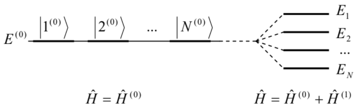Fig. 5.2. Lifting the energy level degeneracy by a perturbation (schematically).

Limiting the summation in Eq. (7) to the group of \(N\) degenerate states with equal \(E_{n}{ }^{(0)} \equiv E^{(0)}\), we reduce it to \[\sum_{n^{n}=1}^{N}\left\langle n^{\prime \prime(0)} \mid n\right\rangle H_{n^{\prime} n^{\prime}}^{(1)}=\left\langle n^{\prime(0)} \mid n\right\rangle\left(E_{n}-E^{(0)}\right),\] where now \(n^{\prime}\) and \(n\) " number the \(N\) states of the degenerate group. \(^{5}\) For \(n=n^{\prime}\), Eq. (24) may be rewritten as \[\sum_{n^{n}=1}^{N}\left(H_{n^{\prime} n^{\prime}}^{(1)}-E_{n^{n}}^{(1)} \delta_{n^{\prime} n^{\prime \prime}}\right)\left(n^{\prime \prime(0)}\left|n^{\prime}\right\rangle=0, \quad \text { where } E_{n}^{(1)} \equiv E_{n}-E^{(0)}\right.\] For each \(n^{\prime}=1,2, \ldots N\), this is a system of \(N\) linear, homogenous equations (with \(N\) terms each) for \(N\) unknown coefficients \(\left\langle n^{\prime,(0)} \mid n^{\prime}\right\rangle\). In this problem, we may readily recognize the problem of diagonalization of the perturbation matrix \(\mathrm{H}^{(1)}-\mathrm{cf}\). Sec. \(4.4\) and in particular Eq. (4.101). As in the general case, the condition of self-consistency of the system is: \[\left|\begin{array}{ccc} H_{11}^{(1)}-E_{n}^{(1)} & H_{12}^{(1)} & \ldots \\ H_{21}^{(1)} & H_{22}^{(1)}-E_{n}^{(1)} & \ldots \\ \ldots & \ldots & \ldots \end{array}\right|=0,\] where now the index \(n\) numbers the \(N\) roots of this equation, in an arbitrary order. According to the definition (25) of \(E_{n}{ }^{(1)}\), the resulting \(N\) energy levels \(E_{n}\) may be found as \(E^{(0)}+E_{n}{ }^{(1)}\). If the perturbation matrix is diagonal in the chosen basis \(n^{(0)}\), the result is extremely simple, \[E_{n}-E^{(0)} \equiv E_{n}^{(1)}=H_{n n}^{(1)},\] and formally coincides with Eq. (14) for the non-degenerate case, but now it may give a different result for each of \(N\) previously degenerate states \(n\).

Now let us see what this general theory gives for several important examples. First of all, let us consider a system with just two degenerate states with energy sufficiently far from all other levels. Then, in the basis of these two degenerate states, the most general perturbation matrix is \[\mathrm{H}^{(1)}=\left(\begin{array}{ll} H_{11} & H_{12} \\ H_{21} & H_{22} \end{array}\right)\] This matrix coincides with the general matrix (5.2) of a two-level system. Hence, we come to the very important conclusion: for a weak perturbation, all properties of any double-degenerate system are identical to those of the genuine two-level systems, which were the subject of numerous discussions in Chapter 4 and again in Sec. 5.1. In particular, its eigenenergies are given by Eq. (5.6), and may be described by the level-anticrossing diagram shown in Fig. 5.1.

---

\({ }^{1}\) Please note the similarity of Eq. (7) with Eq. (2.215) of the 1D band theory. Indeed, the latter equation is not much more than a particular form of Eq. (7) for the 1D wave mechanics, and a specific (periodic) potential \(U(x)\) considered as the perturbation Hamiltonian. Moreover, the whole approximate treatment of the weak-potential limit in Sec. \(2.7\) is essentially a particular case of the perturbation theory we are discussing now (in its \(1^{\text {st }}\) order).

\({ }^{2}\) A useful exercise for the reader: analyze the relation between Eq. (16) and the result of the classical theory of such weakly anharmonic ("nonlinear") oscillator - see, e.g., CM Sec. 5.2, in particular, Eq. (5.49).

\({ }^{3}\) Note that this is correct for the ground-state energy correction \(E_{\mathrm{g}}^{(2)}\) of any system, because for this state, the denominators of all terms of the sum (20) are negative, while their numerators are always non-negative.

\({ }^{4}\) This is exactly the reason why such simple perturbation approach runs into serious problems for systems with a continuous spectrum, and other techniques (such as the WKB approximation) are often necessary.

\({ }^{5}\) Note that here the choice of the basis is to some extent arbitrary, because due to the linearity of equations of quantum mechanics, any linear combination of the states \(n^{\prime \prime(0)}\) is also an eigenstate of the unperturbed Hamiltonian. However, for using Eq. (25), these combinations have to be orthonormal, as was supposed at the derivation of Eq. (7).