6.6: Quantum-mechanical Golden Rule

One of the results of the past section, Eq. (102), may be used to derive one of the most important and nontrivial results of quantum mechanics. For that, let us consider the case when the perturbation causes quantum transitions from a discrete energy level $E_{n}$, into a group of eigenstates with a very dense (essentially continuous) spectrum $E_{n}-$ see Fig. 10a.

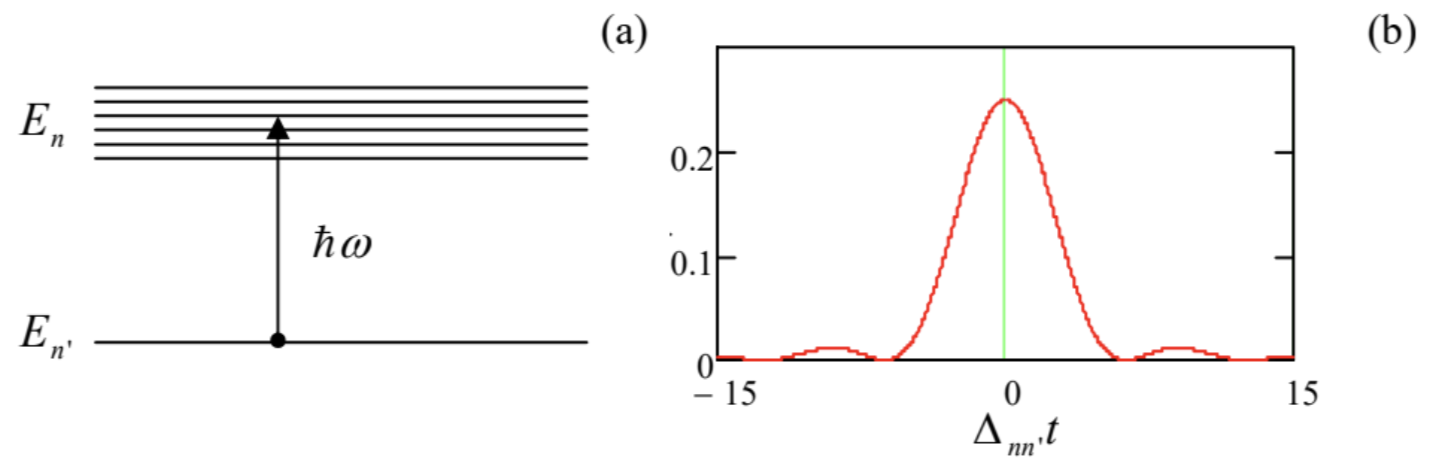Fig. 6.10. Deriving the Golden Rule: (a) the energy level scheme, and (b) the function under the integral (108).

If, for all states $n$ of the group, the following conditions are satisfied $$\left|A_{n n^{\prime}}\right|^{2}<<\left(\hbar \Delta_{n n^{\prime}}\right)^{2}<<\left(\hbar \omega_{n n^{\prime}}\right)^{2},$$ then Eq. (102) coincides with the result that would follow from Eq. (90). This means that we may apply Eq. (102), with the indices $n$ and $n$ ’ duly restored, to any level $n$ of our tight group. As a result, the total probability of having our system transferred from the initial level $n$ ’ to that group is $$W_{\Sigma}(t)=\sum_{n} W_{n}(t)=\frac{4}{\hbar^{2}} \sum_{n} \frac{\left|A_{n n^{\prime}}\right|^{2}}{\Delta_{n n^{\prime}}^{2}} \sin ^{2} \frac{\Delta_{n n} t}{2} .$$ Now comes the main, absolutely beautiful trick: let us assume that the summation over $n$ is limited to a tight group of very similar states whose matrix elements $A_{n n}$ ’ are virtually similar (we will check the validity of this assumption later on), so that we can take $\left|A_{n n}\right|^{2}$ out of the sum in Eq. (107) and then replace the sum with the corresponding integral:

$$W_{\Sigma}(t)=\frac{4\left|A_{n n^{\prime}}\right|^{2}}{\hbar^{2}} \int \frac{1}{\Delta_{n n^{\prime}}^{2}} \sin ^{2} \frac{\Delta_{n n^{\prime}} t}{2} d n \equiv \frac{4\left|A_{n n^{\prime}}\right|^{2} \rho_{n} t}{\hbar} \int \frac{1}{\left(\Delta_{n n^{\prime}} t\right)^{2}} \sin ^{2} \frac{\Delta_{n n^{\prime}} t}{2} d\left(-\Delta_{n n^{\prime}} t\right),$$ where $\rho_{n}$ is the density of the states $n$ on the energy axis: $$\rho_{n} \equiv \frac{d n}{d E_{n}} .$$ This density and the matrix element $A_{n n}$, have to be evaluated at $\Delta_{n n^{\prime}}=0$, i.e. at energy $E_{n}=E_{n^{\prime}}+\hbar \omega$, and are assumed to be constant within the final state group. At fixed $E_{n}$, the function under integral (108) is even and decreases fast at $\left|\Delta_{n n} \cdot t\right|>>1-$ see Fig. 10b. Hence we may introduce a dimensionless integration variable $\xi \equiv \Delta_{n n} \cdot t$, and extend the integration over it formally from $-\infty$ to $+\infty$. Then the integral in Eq. (108) is reduced to a table one, ${ }^{36}$ and yields $$W_{\Sigma}(t)=\frac{4\left|A_{n n^{\prime}}\right|^{2} \rho_{n} t^{+\infty}}{\hbar} \int_{-\infty}^{1} \frac{1}{\xi^{2}} \sin ^{2} \frac{\xi}{2} d \xi=\frac{4\left|A_{n n^{\prime}}\right|^{2} \rho_{n} t}{\hbar} \frac{\pi}{2} \equiv \Gamma t,$$ where the constant $$\Gamma=\frac{2 \pi}{\hbar}\left|A_{n n^{\prime}}\right|^{2} \rho_{n}$$ is called the transition rate. ${ }^{37}$ This is one of the most famous and useful results of quantum mechanics, its Golden Rule $^{38}$, which deserves much discussion.

First of all, let us reproduce the reasoning already used in Sec. $2.5$ to show that the meaning of the rate $\Gamma$ is much deeper than Eq. (110) seems to imply. Indeed, due to the conservation of the total probability, $W_{n}+W_{\Sigma}=1$, we can rewrite that equation as $$\left.\dot{W}_{n^{\prime}}\right|_{t=0}=-\Gamma$$ Evidently, this result cannot be true for all times, otherwise the probability $W_{n}$, would become negative. The reason for this apparent contradiction is that Eq. (110) was obtained in the assumption that initially, the system was completely on level $n^{\prime}: W_{n}(0)=1$. Now, if at the initial moment the value of $W_{n}$, is different, the result (110) has to be multiplied by that number, due to the linear relation (88) between $d a_{n} / d t$ and $a_{n}$. Hence, instead of Eq. (112) we get a differential equation similar to Eq. (2.159), $$\left.\dot{W}_{n^{\prime}}\right|_{t \geq 0}=-\Gamma W_{n^{\prime}},$$ which, for a time-independent $\Gamma$, has the evident solution, $$W_{n^{\prime}}(t)=W_{n^{\prime}}(0) e^{-\Gamma t},$$ describing the exponential decay of the initial state’s occupancy, with the time constant $\tau=1 / \Gamma$.

I am inviting the reader to review this fascinating result again: by the summation of periodic oscillations (102) over many levels $n$, we have got an exponential decay (114) of the probability. This trick becomes possible because the effective range $\Delta E_{n}$ of the state energies $E_{n}$ giving substantial contributions to the integral (108), shrinks with time: $\Delta E_{n} \sim \hbar / t .{ }^{39}$ However, since most of the decay (114) takes place within the time interval of the order of $\tau \equiv 1 / \Gamma$, the range of the participating final energies may be estimated as $$\Delta E_{n} \sim \frac{\hbar}{\tau} \equiv \hbar \Gamma .$$ This estimate is very instrumental for the formulation of conditions of the Golden Rule’s validity. First, we have assumed that the matrix elements of the perturbation and the density of states are independent of the energy within the interval (115). This gives the following requirement $$\Delta E_{n} \sim \hbar \Gamma<<E_{n}-E_{n^{\prime}} \sim \hbar \omega,$$ Second, for the transfer from the sum (107) to the integral (108), we need the number of states within that energy interval, $\Delta N_{n}=\rho_{n} \Delta E_{n}$, to be much larger than 1. Merging Eq. (116) with Eq. (92) for all the energy levels $n^{\prime \prime} \neq n, n^{\prime}$ not participating in the resonant transition, we may summarize all conditions of the Golden Rule validity as $$\rho_{n}^{-1}<<\hbar \Gamma<\hbar\left|\omega \pm \omega_{n^{\prime} n^{\prime \prime}}\right|$$ (The reader may ask whether I have neglected the condition expressed by the first of Eqs. (106). However, for $\Delta_{n n} \sim \Delta E_{n} / \hbar \sim \Gamma$, this condition is just $\left|A_{n n}\right|^{2}<<(\hbar \Gamma)^{2}$, so that plugging it into Eq. (111), $$\Gamma<<\frac{2 \pi}{\hbar}(\hbar \Gamma)^{2} \rho_{n},$$ and canceling one $\Gamma$ and one $\hbar$, we see that it coincides with the first relation in Eq. (117) above.)

Let us have a look at whether these conditions may be satisfied in practice, at least in some cases. For example, let us consider the optical ionization of an atom, with the released electron confined in a volume of the order of $1 \mathrm{~cm}^{3} \equiv 10^{-6} \mathrm{~m}^{3}$. According to Eq. (1.90), with $E$ of the order of the atomic ionization energy $E_{n}-E_{n}=\hbar \omega \sim 1 \mathrm{eV}$, the density of electron states in that volume is of the order of $10^{21} 1 / \mathrm{eV}$, while the right-hand side of Eq. (117) is of the order of $E_{n} \sim 1 \mathrm{eV}$. Thus the conditions (117) provide an approximately 20 -orders-of magnitude range for acceptable values of $\hbar \Gamma$. This illustration should give the reader a taste of why the Golden Rule is applicable to so many situations.

Finally, the physical picture of the initial state’s decay (which will also be the key to our discussion of quantum-mechanical "open" systems in the next chapter) is also very important. According to Eq. (114), the external excitation transfers the system into the continuous spectrum of levels $n$, and it never comes back to the initial level $n$ ’. However, it was derived from the quantum mechanics of Hamiltonian systems, whose equations are invariant with respect to time reversal. This paradox is a result of our generalization (113) of the exact result (112) This trick, breaking the timereversal symmetry, is absolutely adequate for the physics under study. Indeed, some gut feeling of the physical sense of this irreversibility may be obtained from the following observation. As Eq. (1.86) illustrates, the distance between the adjacent orbital energy levels tends to zero only if the system’s size goes to infinity. This means that our assumption of the continuous energy spectrum of the finial states $n$ essentially requires these states to be broadly extended in space - being either free, or essentially free de Broglie waves. Thus the Golden Rule corresponds to the (physically justified) assumption that in an infinitely large system, the traveling de Broglie waves excited by a local source and propagating outward from it, would never come back, and even if they did, unpredictable phase shifts introduced by minor uncontrollable perturbations on their way would never allow them to sum up in the coherent way necessary to bring the system back into the initial state $n$ ’. (This is essentially the same situation which was discussed, for a particular 1D wave-mechanical system, in Sec. 2.5.) $4^{40}$

To get a feeling of the Golden Rule at work, let us apply it to the following simple problem which is a toy model of the photoelectric effect, briefly discussed in Sec. 1.1(ii). A 1D particle is initially trapped in the ground state of a narrow potential well, described by Eq. (2.158): $$U(x)=-W \delta(x), \quad \text { with } w>0 .$$ Let us calculate the rate $\Gamma$ of the particle’s "ionization" (i.e. its excitation into a group of extended, delocalized states) by a weak classical sinusoidal force of amplitude $F_{0}$ and frequency $\omega$, suddenly turned on at some instant, say $t=0$.

As a reminder, the initial localized state (in our current notation, $n$ ’) of such a particle was already found in Sec. 2.6: $$\psi_{n^{\prime}}(x)=\kappa^{1 / 2} \exp \{-\kappa|x|\}, \quad \text { with } \kappa \equiv \frac{m w}{\hbar^{2}}, \quad E_{n^{\prime}} \equiv-\frac{\hbar^{2} \kappa^{2}}{2 m}=-\frac{m w^{2}}{2 \hbar^{2}} .$$ The final, extended states $n$, with a continuous spectrum, for this problem exist only at energies $E_{n}>0$, so that the excitation rate is different from zero only for frequencies $$\omega>\omega_{\min } \equiv \frac{\left|E_{n^{\prime}}\right|}{\hbar}=\frac{m w^{2}}{2 \hbar^{3}} .$$ The weak sinusoidal force may be described by the following perturbation Hamiltonian, $$\hat{H}^{(1)}=-F(t) \hat{x}=-F_{0} \hat{x} \cos \omega t \equiv-\frac{F_{0}}{2} \hat{x}\left(e^{i \omega t}+e^{-i \omega t}\right), \quad \text { for } t>0,$$ so that according to Eq. (86), which serves as the amplitude operator’s definition, in this case $$\hat{A}=\hat{A}^{\dagger}=-\frac{F_{0}}{2} \hat{x} .$$ The matrix elements $A_{n n}$, that participate in Eq. (111) may be readily calculated in the coordinate representation:

$$A_{n n^{\prime}}=\int_{-\infty}^{+\infty} \psi_{n}^{*}(x) \hat{A}(x) \psi_{n^{\prime}}(x) d x=-\frac{F_{0}}{2} \int_{-\infty}^{+\infty} \psi_{n}^{*}(x) x \psi_{n^{\prime}}(x) d x .$$ Since, according to Eq. (120), the initial $\psi_{n}$ ’ is a symmetric function of $x$, non-vanishing contributions to this integral are given only by antisymmetric functions $\psi_{n}(x)$, proportional to $\sin k_{n} x$, with the wave number $k_{n}$ related to the final energy by the well-familiar equality (1.89): $$\frac{\hbar^{2} k_{n}^{2}}{2 m}=E_{n} .$$ As we know from Sec. $2.6$ (see in particular Eq. (2.167) and its discussion), such antisymmetric functions, with $\psi_{n}(0)=0$, are not affected by the zero-centered delta-functional potential (119), so that their density $\rho_{n}$ is the same as that in completely free space, and we could use Eq. (1.100). However, since that relation was derived for traveling waves, it is more prudent to repeat its derivation for standing waves, confining them to an artificial segment $[-l / 2,+l / 2]-$ long in the sense $$k_{n} l, \kappa l>>1 \text {, }$$ so it does not affect the initial localized state and the excitation process. Then the confinement requirement $\psi_{n}(\pm l / 2)=0$ immediately yields the condition $k_{n} l / 2=n \pi$, so that Eq. (1.100) is indeed valid, but only for positive values of $k_{n}$, because $\sin k_{n} x$ with $k_{n} \rightarrow-k_{n}$ does not describe an independent standing-wave eigenstate. Hence the final state density is $$\rho_{n} \equiv \frac{d n}{d E_{n}} \equiv \frac{d n}{d k_{n}} / \frac{d E_{n}}{d k_{n}}=\frac{l}{2 \pi} / \frac{\hbar^{2} k_{n}}{m} \equiv \frac{l m}{2 \pi \hbar^{2} k_{n}} .$$ It may look troubling that the density of states depends on the artificial segment’s length $l$, but the same $l$ also participates in the final wavefunctions’ normalization factor, ${ }^{41}$ $$\psi_{n}=\left(\frac{2}{l}\right)^{1 / 2} \sin k_{n} x \text {, }$$ and hence in the matrix element (124): $$A_{n n^{\prime}}=-\frac{F_{0}}{2}\left(\frac{2 \kappa}{l}\right)^{1 / 2} \int_{-l}^{+l} \sin k_{n} x e^{-\kappa|x|} x d x .=-\frac{F_{0}}{2 i}\left(\frac{2 \kappa}{l}\right)^{1 / 2}\left(\int_{0}^{l} e^{\left(i k_{n}-\kappa\right) x} x d x-\int_{0}^{l} e^{-\left(i k_{n}+\kappa\right) x} x d x\right) .$$ These two integrals may be readily worked out by parts. Taking into account that due to the condition (126), their upper limits may be extended to $\infty$, the result is $$A_{n n^{\prime}}=-\left(\frac{2 \kappa}{l}\right)^{1 / 2} F_{0} \frac{2 k_{n} \kappa}{\left(k_{n}^{2}+\kappa^{2}\right)^{2}} .$$ Note that the matrix element is a smooth function of $k_{n}$ (and hence of $E_{n}$ ), so that an important condition of the Golden Rule, the virtual constancy of $A_{n n}$ ’ on the interval $\Delta E_{n} \sim \hbar \Gamma<<E_{n}$, is satisfied. So, the general Eq. (111) is reduced, for our problem, to the following expression:

$$\Gamma=\frac{2 \pi}{\hbar}\left[\left(\frac{2 \kappa}{l}\right)^{1 / 2} F_{0} \frac{2 k_{n} \kappa}{\left(k_{n}^{2}+\kappa^{2}\right)^{2}}\right]^{2} \frac{l m}{2 \pi \hbar^{2} k_{n}} \equiv \frac{8 F_{0}^{2} m k_{n} \kappa^{3}}{\hbar^{3}\left(k_{n}^{2}+\kappa^{2}\right)^{4}},$$ which is independent of the artificially introduced $l$ - thus justifying its use.

Note that due to the above definitions of $k_{n}$ and $\kappa$, the expression in the parentheses in the denominator of the last expression does not depend on the potential well’s "weight" $w$, and is a function of only the excitation frequency $\omega$ (and the particle’s mass): $$\frac{\hbar^{2}\left(k_{n}^{2}+\kappa^{2}\right)}{2 m}=E_{n}-E_{n^{\prime}}=\hbar \omega \text {. }$$ As a result, Eq. (131) may be recast simply as $$\hbar \Gamma=\frac{F_{0}^{2} w^{3} k_{n}}{2(\hbar \omega)^{4}} .$$ What is hidden here is that $k_{n}$, defined by Eq. (125) with $E_{n}=E_{n}{ }^{\prime}+\hbar \omega$, is a function of the external force’s frequency, changing as $\omega^{1 / 2}$ at $\omega>>\omega_{\min }$ (so that $\Gamma$ drops as $\omega^{-7 / 2}$ at $\omega \rightarrow \infty$ ), and as $\left(\omega-\omega_{\min }\right)^{1 / 2}$ when $\omega$ approaches the "red boundary" (121) of the ionization effect, so that $\Gamma \propto\left(\omega-\omega_{\min }\right)^{1 / 2} \rightarrow 0$ in that limit as well.

A conceptually very similar, but a bit more involved analysis of such effect in a more realistic 3D case, namely the hydrogen atom’s ionization by an optical wave, is left for the reader’s exercise.

---

${ }^{36}$ See, e.g., MA Eq. (6.12).

${ }^{37}$ In some texts, the density of states in Eq. (111) is replaced with a formal expression $\sum \delta\left(E_{n}-E_{n^{\prime}}-\hbar \omega\right)$. Indeed, applied to a finite energy interval $\Delta E_{n}$ with $\Delta n \gg 1$ levels, it gives the same result: $\Delta n \equiv\left(d n / d E_{n}\right) \Delta E_{n} \equiv \rho_{n} \Delta E_{n}$. Such replacement may be technically useful in some cases, but is incorrect for $\Delta n \sim 1$, and hence should be used with the utmost care, so that for most applications the more explicit form (111) is preferable.

${ }^{38}$ Sometimes Eq. (111) is called "Fermi’s Golden Rule". This is rather unfair, because this result was developed mostly by the same P. A. M. Dirac in 1927, and Enrico Fermi’s role was not much more than advertising it, under the name of "Golden Rule No. 2", in his influential lecture notes on nuclear physics, which were published much later, in 1950. (To be fair to Fermi, he has never tried to pose as the Golden Rule’s author.)

${ }^{39}$ This is one more appearance of the "energy-time uncertainty relation", which was discussed in Sec. $2.5$.

${ }^{40}$ This situation is also similar to the irreversible increase of entropy of macroscopic systems, despite the fact that their microscopic components obey reversible laws of motion, which is postulated in thermodynamics and explained in statistical physics - see, e.g., SM Secs. $1.2$ and $2.2 .$

${ }^{41}$ The normalization to infinite volume, using Eq. (4.263), is also possible, but physically less transparent.