6.5: Time-dependent Perturbations

Now let us proceed to the case when the perturbation \(\hat{H}^{(1)}\) in Eq. (1) is a function of time, while \(\hat{H}^{(0)}\) is time-independent. The adequate perturbative approach to this problem, and its results, depend critically on the relation between the characteristic frequency \(\omega\) of the perturbation and the distance between the initial system’s energy levels: \[\hbar \omega \leftrightarrow\left|E_{n}-E_{n^{\prime}}\right| .\] In the case when all essential frequencies of a perturbation are very small in the sense of Eq. (74), we are dealing with the so-called adiabatic change of parameters, that may be treated essentially as a time-independent perturbation - see the previous sections of this chapter). The most interesting observation here is that the adiabatic perturbation does not allow any significant transfer of system’s probability from one eigenstate to another. For example, in the WKB limit of the orbital motion, the Bohr quantization rule and its Wilson-Sommerfeld modification (2.110) guarantee that the integral \[\oint_{C} \mathbf{p} \cdot d \mathbf{r},\] taken along the particle’s classical trajectory, is an adiabatic invariant, i.e. does not change at a slow change of system’s parameters. (It is curious that classical mechanics also guarantees the invariance of the integral (75), but its proof there \({ }^{23}\) is much harder than the quantum-mechanical derivation of this fact, carried out in Sec. 2.4.) This is why even if the perturbation becomes large with time (while changing sufficiently slowly), we can expect the classification of eigenstates and eigenvalues to persist.

Let us proceed to the harder case when both sides of Eq. (74) are comparable, using for this discussion the Schrödinger picture of quantum dynamics, given by Eq. (4.158). Combining it with Eq. (1), we get the Schrödinger equation in the form \[i \hbar \frac{\partial}{\partial t}|\alpha(t)\rangle=\left(\hat{H}^{(0)}+H^{(1)}(t)\right)|\alpha(t)\rangle .\] Very much in the spirit of our treatment of the time-independent case in Sec. 1, let us represent the timedependent ket-vector of the system with its expansion, \[|\alpha(t)\rangle=\sum_{n}|n\rangle\langle n \mid \alpha(t)\rangle,\] over the full and orthonormal set of the unperturbed, stationary ket-vectors defined by equation \[\hat{H}^{(0)}|n\rangle=E_{n}|n\rangle\] (Note that these kets \(|n\rangle\) are exactly what was called \(\left|n^{(0)}\right\rangle\) in Sec. 1; we may afford a less bulky notation in this section, because only the lowest orders of the perturbation theory will be discussed.) Plugging the expansion (77), with \(n\) replaced with \(n\) ’, into both sides of Eq. (76), and then inner-multiplying both its sides by the bra-vector \(\langle n|\) of another unperturbed (and hence time-independent) state of the system, we get the following set of linear, ordinary differential equations for the expansion coefficients: \[i \hbar \frac{d}{d t}\langle n \mid \alpha(t)\rangle=E_{n}\langle n \mid \alpha(t)\rangle+\sum_{n^{\prime}} H_{n n^{\prime}}^{(1)}(t)\left\langle n^{\prime} \mid \alpha(t)\right\rangle,\] where the matrix elements of the perturbation, in the unperturbed state basis, defined similarly to Eq. (8), are now functions of time: \[H_{n n^{\prime}}^{(1)}(t) \equiv\left\langle n\left|\hat{H}^{(1)}(t)\right| n^{\prime}\right\rangle .\] The set of differential equations (79), which are still exact, may be useful for numerical calculations. \({ }^{24}\) However, it has a certain technical inconvenience, which becomes clear if we consider its (evident) solution in the absence of perturbation: \({ }^{25}\)

\[\langle n \mid \alpha(t)\rangle=\langle n \mid \alpha(0)\rangle \exp \left\{-i \frac{E_{n}}{\hbar} t\right\} .\] We see that these solutions oscillate very fast, and their numerical modeling may represent a challenge for even the fastest computers. These spurious oscillations (whose frequency, in particular, depends on the energy reference level) may be partly tamed by looking for the general solution of Eqs. (79) in a form inspired by Eq. (81): \[\langle n \mid \alpha(t)\rangle \equiv a_{n}(t) \exp \left\{-i \frac{E_{n}}{\hbar} t\right\} .\] Here \(a_{n}(t)\) are new functions of time (essentially, the stationary states’ probability amplitudes), which may be used, in particular, to calculate the time-dependent level occupancies, i.e. the probabilities \(W_{n}\) to find the perturbed system on the corresponding energy levels of the unperturbed system: \[W_{n}(t)=|\langle n \mid \alpha(t)\rangle|^{2}=\left|a_{n}(t)\right|^{2} .\]

Plugging Eq. (82) into Eq. (79), for these functions we readily get a slightly modified system of equations: \[i \hbar \dot{a}_{n}=\sum_{n^{\prime}} a_{n^{\prime}} H_{n n^{\prime}}^{(1)}(t) e^{i \omega_{n n^{\prime}} t},\] where the factors \(\omega_{n n}\), defined by the relation \[\hbar \omega_{n n^{\prime}} \equiv E_{n}-E_{n^{\prime}},\] have the physical sense of frequencies of potential quantum transitions between the \(n^{\text {th }}\) and \(n^{, \text {th }}\) energy levels of the unperturbed system. (The conditions when such transitions indeed take place will be clear soon.) The advantages of Eq. (84) over Eq. (79), for both analytical and numerical calculations, is their independence of the energy reference, and lower frequencies of oscillations of the right-hand side terms, especially when the energy levels of interest are close to each other. \({ }^{26}\)

In order to continue our analytical treatment, let us focus on a particular but very important problem of a sinusoidal perturbation turned on at some moment \(-\) which may be taken for \(t=0\) : \[\hat{H}^{(1)}(t)= \begin{cases}0, & \text { for } t<0, \\ \hat{A} e^{-i \omega t}+\hat{A}^{\dagger} e^{+i \omega t}, & \text { for } t \geq 0,\end{cases}\]

where the perturbation amplitude operators \(\ \hat{A}\) and \(\ \hat{A}^{\dagger}\),²⁷ and hence their matrix elements,

\[\ \left\langle n|\hat{A}| n^{\prime}\right\rangle \equiv A_{n n^{\prime}}, \quad\left\langle n\left|\hat{A}^{\dagger}\right| n^{\prime}\right\rangle=A_{n^{\prime} n}^{*},\]

are time-independent after the turn-on moment. In this case, Eq. (84) yields

\[\ i \hbar \dot{a}_{n}=\sum_{n^{\prime}} a_{n^{\prime}}\left[A_{n n^{\prime}} e^{i\left(\omega_{n n^{\prime}}-\omega\right) t}+A_{n^{\prime} n}^{*} e^{i\left(\omega_{n n^{\prime}}+\omega\right) t}\right], \quad \text { for } t>0 .\]

This is, generally, still a nontrivial system of coupled differential equations; however, it allows simple and explicit solutions in two very important limits. First, let us assume that our system initially was definitely in one eigenstate \(\ n^{\prime}\) (usually, though not necessarily, in the ground state), and that the occupancies \(\ W_{n}\) of all other levels stay very low all the time. (We will find the condition when the second assumption is valid a posteriori – from the solution.) With these assumptions,

\[\ a_{n^{\prime}}=1 ; \quad\left|a_{n}\right|<<1, \quad \text { for } n \neq n^{\prime},\]

Eq. (88) may be readily integrated, giving

\[\ a_{n}=-\frac{A_{n n^{\prime}}}{\hbar\left(\omega_{n n^{\prime}}-\omega\right)}\left[e^{i\left(\omega_{n n^{\prime}}-\omega\right) t}-1\right]-\frac{A_{n^{\prime} n}^{*}}{\hbar\left(\omega_{n n^{\prime}}+\omega\right)}\left[e^{i\left(\omega_{n n^{\prime}}+\omega\right) t}-1\right], \quad \text { for } n \neq n^{\prime} .\]

This expression describes what is colloquially called the ac excitation of (other) energy levels. Qualitatively, it shows that the probability \(\ W_{n}\) (83) of finding the system in each state (“on each energy level”) of the system does not tend to any constant value but rather oscillates in time. It also shows that that the ac-field-induced transfer of the system from one state to the other one has a clearly resonant character: the maximum occupancy \(\ W_{n}\) of a level number \(\ n \neq n^{\prime}\) grows infinitely when the corresponding detuning²⁸

\[\ \Delta_{n n^{\prime}} \equiv \omega-\omega_{n n^{\prime}},\]

tends to zero. This conclusion is clearly unrealistic, and is an artifact of our initial assumption (89); according to Eq. (90), it is satisfied only if²⁹

\[\ \left|A_{n n^{\prime}}\right|<<\hbar\left|\omega \pm \omega_{n n^{\prime}}\right|,\]

and hence which does not allow a more deep analysis of the resonant excitation.

In order to overcome this limitation, we may perform the following trick - very similar to the one we used for the transfer to the degenerate case in Sec. 1. Let us assume that for a certain level \(n\), \[\left|\Delta_{n n^{\prime}}\right|<<\omega,\left|\omega \pm \omega_{n^{\prime \prime} n}\right|,\left|\omega \pm \omega_{n^{\prime \prime} n^{\prime}}\right|, \quad \text { for all } n^{\prime \prime} \neq n, n^{\prime}\]

• the condition illustrated in Fig. 8. Then, according to Eq. (90), we may ignore the occupancy of all but two levels, \(n\) and \(n^{\prime}\), and also the second, non-resonant term with frequency \(\omega_{n n^{\prime}}+\omega \approx 2 \omega>>\left|\Delta_{n n}\right|\) in Eqs. (88), \({ }^{30}\) now written for two probability amplitudes, \(a_{n}\) and \(a_{n}\).

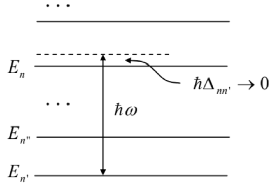Fig. 6.8. The resonant excitation of an energy level.

The result is the following system of two linear equations: \[i \hbar \dot{a}_{n}=a_{n^{\prime}} A e^{-i \Delta t}, \quad i \hbar \dot{a}_{n^{\prime}}=a_{n} A^{*} e^{i \Delta t},\] which uses the shorthand notation \(A \equiv A_{n n}\) ’ and \(\Delta \equiv \Delta_{n n}\). (I will use this notation for a while - until other energy levels become involved, at the beginning of the next section). This system may be readily reduced to a form without explicit time dependence of the right-hand parts - for example, by introducing the following new probability amplitudes, with the same moduli: \[b_{n} \equiv a_{n} e^{i \Delta t / 2}, \quad b_{n^{\prime}} \equiv a_{n^{\prime}} e^{-i \Delta t / 2},\] so that \[a_{n}=b_{n} e^{-i \Delta t / 2}, \quad a_{n^{\prime}}=b_{n^{\prime}} e^{i \Delta t / 2} .\] Plugging these relations into Eq. (94), we get two usual linear first-order differential equations: \[i \hbar \dot{b}_{n}=-\frac{\hbar \Delta}{2} b_{n}+A b_{n^{\prime}}, \quad i \hbar \dot{b}_{n^{\prime}}=A^{*} b_{n}+\frac{\hbar \Delta}{2} b_{n^{\prime}} .\] As the reader knows very well by now, the general solution of such a system is a linear combination of two exponential functions, \(\exp \left\{\lambda_{\pm} t\right\}\), with the exponents \(\lambda_{\pm}\)that may be found by plugging any of these functions into Eq. (97), and requiring the consistency of the two resulting linear algebraic equations. In our case, the consistency condition (i.e. the characteristic equation of the system) is \[\left|\begin{array}{cc} -\hbar \Delta / 2-i \hbar \lambda & A \\ A^{*} & \hbar \Delta / 2-i \hbar \lambda \end{array}\right|=0,\] and has two solutions \(\lambda_{\pm}=\pm i \Omega\), where \[\Omega \equiv\left(\frac{\Delta^{2}}{4}+\frac{|A|^{2}}{\hbar^{2}}\right)^{1 / 2}, \quad \text { i.e. } 2 \Omega=\left(\Delta^{2}+4 \frac{|A|^{2}}{\hbar^{2}}\right)^{1 / 2}\] The coefficients at the exponents are determined by initial conditions. If, as was assumed before, the system was completely on the level \(n^{\prime}\) initially (at \(t=0\) ), i.e. if \(a_{n^{\prime}}(0)=1, a_{n}(0)=0\), so that \(b_{n^{\prime}}(0)=\) \(1, b_{n}(0)=0\) as well, then Eqs. (97) yield, in particular: \[b_{n}(t)=-i \frac{A}{\hbar \Omega} \sin \Omega t,\] so that the \(n^{\text {th }}\) level occupancy is \[W_{n}=\left|b_{n}\right|^{2}=\frac{|A|^{2}}{\hbar^{2} \Omega^{2}} \sin ^{2} \Omega t \equiv \frac{|A|^{2}}{|A|^{2}+(\hbar \Delta / 2)^{2}} \sin ^{2} \Omega t .\] This is the famous Rabi oscillation formula \({ }^{31}\) If the detuning is large in comparison with \(|A| / \hbar\), though still small in the sense of Eq. (93), the frequency \(2 \Omega\) of the Rabi oscillations is completely determined by the detuning, and their amplitude is small: \[W_{n}(t)=4 \frac{|A|^{2}}{\hbar^{2} \Delta^{2}} \sin ^{2} \frac{\Delta t}{2}<<1, \quad \text { for }|A|^{2}<<(\hbar \Delta)^{2},\]

• the result which could be obtained directly from Eq. (90), just neglecting the second term on its righthand side. However, now we may also analyze the results of an increase of the perturbation amplitude: it leads not only to an increase of the amplitude of the probability oscillations, but also of their frequency - see Fig. 9. Ultimately, at \(|A| \gg>\hbar|\Delta|\) (for example, at the exact resonance, \(\Delta=0\)., i.e. \(\omega_{n n}{ }^{\prime}=\omega\), so that \(\left.E_{n}=E_{n^{\prime}}+\hbar \omega\right)\), Eqs. (101)-(102) give \(\Omega=|A| / \hbar\) and \(\left(W_{n}\right)_{\max }=1\), i.e. describe a periodic, full "repumping" of the system from one level to another and back, with a frequency proportional to the perturbation amplitude. \({ }^{32}\)

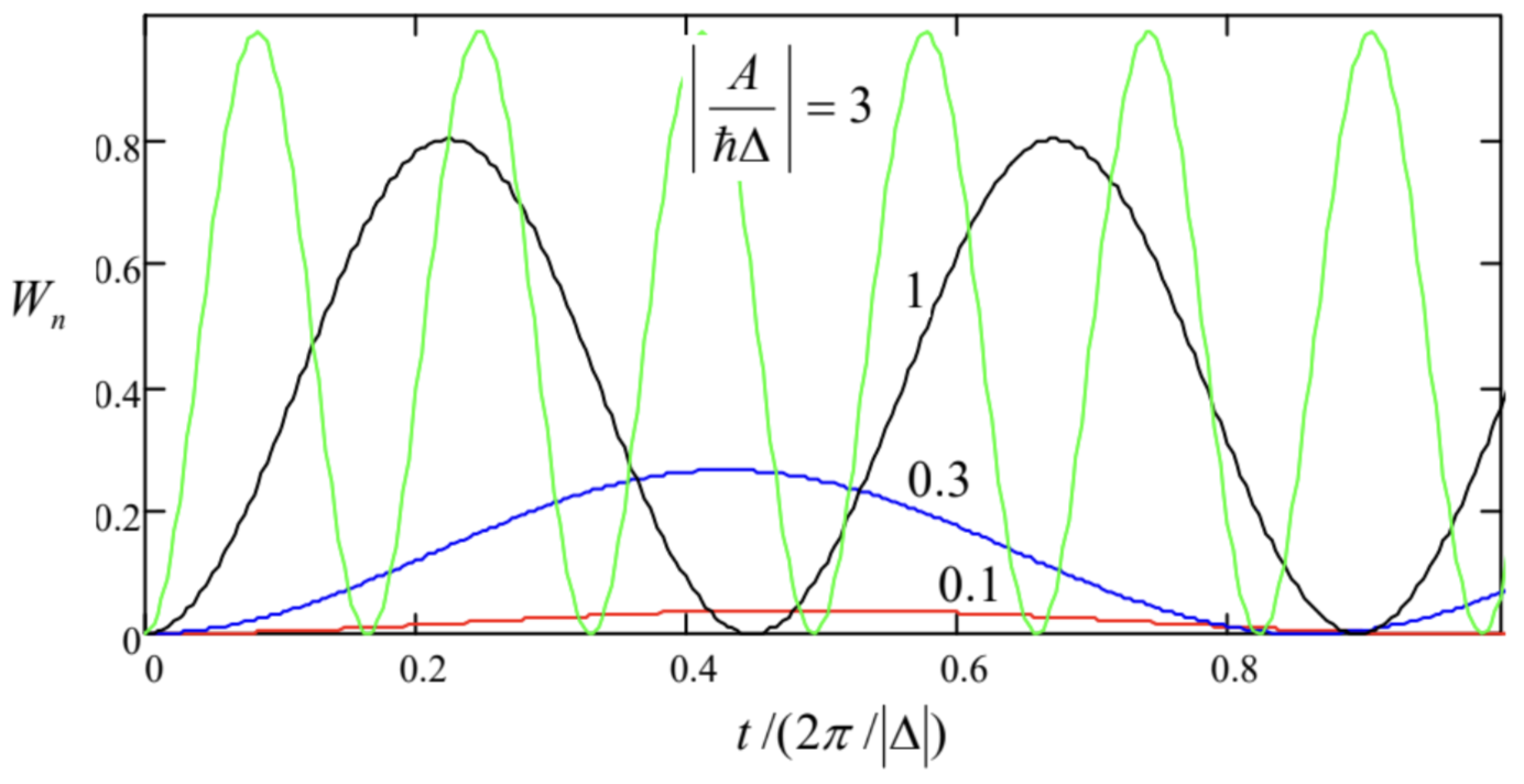Fig. 6.9. The Rabi oscillations for several values of the normalized amplitude of ac perturbation.

This effect is a close analog of the quantum oscillations in two-level systems with timeindependent Hamiltonians, which were discussed in Secs. \(2.6\) and 5.1. Indeed, let us revisit, for a moment, their discussion started at the end of Sec.1 of this chapter, now paying more attention to the time evolution of the system under the perturbation. As was argued in that section, the most general perturbation Hamiltonian lifting the two-fold degeneracy of an energy level, in an arbitrary basis, has the matrix (28). Let us describe the system’s dynamics using, again, the Schrödinger picture, representing the ket-vector of an arbitrary state of the system in the form (5.1), where \(\uparrow\) and \(\downarrow\) are the time-independent states of the basis in that Eq. (28) is written (now without any obligation to associate these states with the \(z\)-basis of any spin- \(1 / 2 .\) ) Then, the Schrödinger equation (4.158) yields \[i \hbar\left(\begin{array}{l} \dot{\alpha}_{\uparrow} \\ \dot{\alpha}_{\downarrow} \end{array}\right)=\mathrm{H}^{(1)}\left(\begin{array}{l} \alpha_{\uparrow} \\ \alpha_{\downarrow} \end{array}\right) \equiv\left(\begin{array}{ll} H_{11} & H_{12} \\ H_{21} & H_{22} \end{array}\right)\left(\begin{array}{l} \alpha_{\uparrow} \\ \alpha_{\downarrow} \end{array}\right) \equiv\left(\begin{array}{l} H_{11} \alpha_{\uparrow}+H_{12} \alpha_{\downarrow} \\ H_{21} \alpha_{\uparrow}+H_{22} \alpha_{\downarrow} \end{array}\right) .\] As we know (for example, from the discussion in Sec. 5.1), the average of the diagonal elements of the matrix gives just a common shift of the system’s energy; for the purpose of the dynamics analysis, it may be absorbed into the energy reference level. Also, the Hamiltonian operator has to be Hermitian, so that the off-diagonal elements of its matrix have to be complex-conjugate. With this, Eqs. (103) are reduced to the form, \[i \hbar \dot{\alpha}_{\uparrow}=-\frac{\xi}{2} \alpha_{\uparrow}+H_{12} \alpha_{\downarrow}, \quad i \hbar \dot{\alpha}_{\downarrow}=H_{12}^{*} \alpha_{\uparrow}+\frac{\xi}{2} \alpha_{\downarrow}, \quad \text { with } \hbar \xi \equiv H_{22}-H_{11},\] which is absolutely similar to Eqs. (97). In particular, these equations describe the quantum oscillations of the probabilities \(W_{\uparrow}=|\alpha \uparrow|^{2}\) and \(W_{\downarrow}=|\alpha \downarrow|^{2}\) with the frequency \(^{33}\) \[2 \Omega=\left(\xi^{2}+4 \frac{\left|H_{12}\right|^{2}}{\hbar^{2}}\right)^{1 / 2} .\] The similarity of Eqs. (97) and (104), and hence of Eqs. (99) and (105), shows that the "usual" quantum oscillations and the Rabi oscillations have essentially the same physical nature, besides that in the latter case the external ac signal quantum \(\hbar \omega\) bridges the separated energy levels, effectively reducing their difference \(\left(E_{n}-E_{n}^{\prime}\right)\) to a much smaller difference \(-\Delta \equiv\left(E_{n}-E_{n}^{\prime}\right)-\hbar \omega\). Also, since the Hamiltonian (28) is similar to that given by Eq. (5.2), the dynamics of such a system with two accoupled energy levels, within the limits (93) of the perturbation theory, is completely similar to that of a time-independent two-level system. In particular, its state may be similarly represented by a point on the Bloch sphere shown in Fig. 5.3, with its dynamics described, in the Heisenberg picture, by Eq. (5.19). This fact is very convenient for the experimental implementation of quantum information systems (to be discussed in more detail in Sec. 8.5), because it enables qubit manipulations in a broad variety of physical systems with well-separated energy levels, using external ac (usually either microwave or optical) sources.

Note, however, that according to Eq. (90), if the system has energy levels other than \(n\) and \(n\) ’, they also become occupied to some extent. Since the sum of all occupancies equals 1, this means that \(\left(W_{n}\right)_{\max }\) may approach 1 only if the other excitation amplitude is very small, and hence the state manipulation time scale \(\tau=2 \pi / \Omega=2 \pi \hbar /|A|\) is very long. The ultimate limit in this sense is provided by the harmonic oscillator where all energy levels are equidistant, and the probability repumping between all of them occurs at comparable rates. In particular, in this system the implementation of the full Rabi oscillations is impossible even at the exact resonance. \({ }^{34}\)

However, I would not like these the quantitative details to obscure from the reader the most important qualitative (OK, maybe semi-quantitative :-) conclusion of this section’s analysis: a resonant increase of the interlevel transition intensity at \(\omega \rightarrow \omega_{n n}\). As will be shown later in the course, in a quantum system coupled to its environment at least slightly (hence in reality, in any quantum system), such increase is accompanied by a sharp increase of the external field’s absorption, which may be measured. This effect has numerous practical applications including spectroscopies based on the electron paramagnetic resonance (EPR) and nuclear magnetic resonance (NMR), which are broadly used in material science, chemistry, and medicine. Unfortunately, I will not have time to discuss the related technical issues and methods (in particular, interesting ac pulsing techniques, including the so-called Ramsey interferometry) in detail, and have to refer the reader to special literature. \({ }^{35}\)

---

\({ }^{23}\) See, e.g., CM Sec. 10.2.

\({ }^{24}\) Even if the problem under analysis may be described by the wave-mechanics Schrödinger equation (1.25), a direct numerical integration of that partial differential equation is typically less convenient than that of the ordinary differential equations (79).

\({ }^{25}\) This is of course just a more general form of Eq. (1.62) of the wave mechanics of time-independent systems.

\({ }^{26}\) Note that the relation of Eq. (84) to the initial Eq. (79) is very close to the relation of the interaction picture of quantum dynamics, discussed at the end of Sec. 4.6, to its Schrödinger picture, with the perturbation Hamiltonian playing the role of the interaction one - compare Eqs. (1) and Eq. (4.206). Indeed, Eq. (84) could be readily obtained from the interaction picture, and I did not do this just to avoid using this heavy bra-ket artillery for our current (relatively) simple problem, and hence to keep its physics more transparent.

\({ }_{27}\) The notation of the amplitude operators in Eq. (86) is justified by the fact that the perturbation Hamiltonian has to be self-adjoint (Hermitian), and hence each term on the right-hand side of that relation has to be a Hermitian conjugate of its counterpart, which is evidently true only if the amplitude operators are also the Hermitian conjugates of each other. Note, however, that each of these amplitude operators is generally not Hermitian.

\({ }^{28}\) The notion of detuning is also very useful in the classical theory of oscillations (see, e.g., CM Chapter 5 ), where the role of \(\omega_{n n}\) is played by the own frequency \(\omega_{0}\) of the oscillator.

\({ }^{29}\) Strictly speaking, one more condition is that the number of "resonance" levels is also not too high - see Sec. 6 .

\({ }^{30}\) The second assumption, i.e. the omission of non-resonant terms in the equations for amplitudes is called the Rotating Wave Approximation (RWA); the same idea in the classical theory of oscillations is the basis of what is usually called the van der Pol method, and its result, the reduced equations - see, e.g., CM Secs. 5.3-5.5.

\({ }^{31}\) It was derived in 1952 by Isaac Rabi, in the context of his group’s pioneering experiments with the ac (practically, microwave) excitation of quantum states, using molecular beams in vacuum.

\({ }^{32}\) As Eqs. (82), (96), and (99) show, the lowest frequency in the system is \(\omega_{1}=\omega_{n^{\prime}}-\Delta / 2+\Omega\), so that at \(A \rightarrow 0\), \(\hbar \omega_{1} \approx \omega_{n^{\prime}}+2|A|^{2} / \hbar \Delta\). This effective shift of the lowest energy level (which may be measured by another "probe" field of a different frequency) is a particular case of the ac Stark effect, which was already mentioned in Sec. 2 .

\({ }^{33}\) By the way, Eq. (105) gives a natural generalization of the relations obtained for the frequency of such oscillations in Sec. 2.6, where the coupled potential wells were assumed to be exactly similar, so that \(\xi=0\). Moreover, Eqs. (104) gives a long-promised proof of Eqs. (2.201), and hence a better justification of Eqs. (2.203).

\({ }^{34}\) From Sec. 5.5, we already know what happens to the ground state of an oscillator at its external sinusoidal (or any other) excitation: it turns into a Glauber state, i.e. a superposition of all Fock states - see Eq. (5.134).

\({ }^{35}\) For introductions see, e.g., J. Wertz and J. Bolton, Electron Spin Resonance, \(2^{\text {nd }}\) ed., Wiley, 2007; J. Keeler, Understanding NMR Spectroscopy, \(2^{\text {nd }}\) ed., Wiley, \(2010 .\)