11.9: Magnetic Induction

What Is Induction?

We have seen how Ørsted was able to demonstrate that electric currents can produce magnetic fields. The English physicist Michael Faraday, a brilliant experimentalist, was the first to demonstrate the converse effect just a few years later in 1831: magnetic fields can be used to induce electric currents. This is now called the principle of magnetic induction. It is interesting to note that Faraday had little formal schooling, so mathematics was by no means his strength. Nevertheless, he was one of the most influential scientists not just of his time, but his contributions continue to find applications to this day.

For example, when he demonstrated that magnetic fields could be used to produce a current in a wire loop, politicians at the time were not impressed as they failed to see the use of it. It turns out that this was the critical step in creating generators and power plants, which make electricity available without flying a kite in a storm or carrying large arrays of batteries. The alternating-current (AC) circuits that power all the electrical grids of the world have as part of their components a generator that is based on magnetic induction.

More recently, highly fuel efficient vehicles such as the gas-electric hybrid cars employ a technology called regenerative braking. This uses a device that can give power to the wheels of the car by means of an electric battery, and can recharge the battery during braking by running the circuit in “reverse”, transforming the kinetic energy of the car’s motion into electric potential energy stored in the battery and saving fuel as a result. This recent application has large implications for the world’s economy and is of global environmental impact, and at its core lies Faraday’s principle of induction: that we can transform magnetic fields to electric currents.

Magnetic Flux

Before we tackle the principle of magnetic induction, we first need to define a quantity which is crucial to understand it quantitatively: the concept of magnetic flux.

Let us discuss first the idea of flux in general using a familiar example: rain falling on the windshield of a car. Suppose that we want to quantitatively determine the amount of rain that hits the windshield of the car. For simplicity, first assume that the rain is falling vertically down, and that the shape of the windshield is a rectangle. Let us further simplify by assuming you are in a parked car, i.e. it is not moving. If we want to find how much rain hits the windshield, we mainly need to consider these three variables:

• The amount of rain
• The size of the windshield
• The orientation of the windshield relative to the rain

Let’s discuss each in turn. If it is raining hard, there will be a lot more raindrops hitting the windshield than if it is raining lightly. Likewise, If the size of the windshield is large, more raindrops will hit it than if it were small. The orientation between the rain and the windshield will also determine how much rain hits the windshield: if the windshield were arranged vertically, there would be no rain hitting the windshield (in the idealization that the windshield is infinitely thin). Conversely, the most amount of rain will hit if it's arranged perpendicular to the rain, or horizontally (like the sunroof on top of the car). In general, the flux of some quantity through a surface area is a measure of how much of that quantity passes through the area.

This idea of calculating the amount of rain hitting a surface is analogous the concept of magnetic flux, \(\Phi\). We can consider the flux of the magnetic field passing through an arbitrarily-chosen surface. In our example, the rain falling vertically is our vector field, and the windshield is our arbitrary area. More rain means that the magnitude, \(|\vec B|\), of the vector field increases. A larger windshield means a greater surface area. The orientation is measured by the angle between the direction of the vector field and the normal vector, \(\hat n\), to the surface area. The normal vector is a unit vector which is perpendicular to the surface through which flux is being calculated. For the particular case of the magnetic field vector \(\vec{B}\), we define the magnetic flux \(\Phi\) through an area \(A\) as:

\[\Phi = \vec B\cdot A\hat n = |\vec{B}||A| \cos \theta\label{flux}\]

where the angle \(\theta\) is the angle between the magnetic field vector, \(\vec B\) and the vector normal, \(\hat n\) to the surface area \(A\), as depicted in the figure below, for some arbitrary alignment of the magnetic field with a surface represented by a plane.

Figure 11.9.1: Magnetic Flux

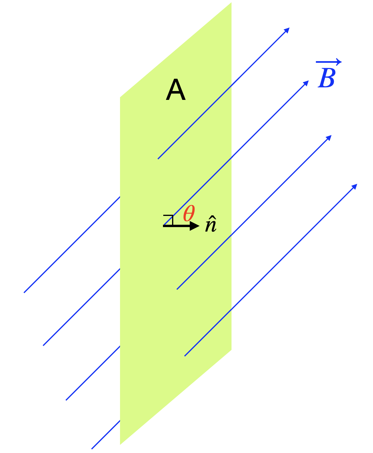
From our rain example, you can see that when the rain is falling vertically down, and the windshield surface is horizontal, the normal vector to the area will be vertical. Hence, the rain and the normal vector are parallel to each other, and the angle in Equation \ref{flux} will be \(\theta = 0^{\circ}\). Since \(\cos\theta = 1\), this orientation maximizes flux. If the windshield surface is vertical, the vector normal to the surface area will now be horizontal, the angle will be \(\theta = 90°\), resulting in \(\cos \theta = 0\) and the flux will vanish (no rain hits the vertical windshield). Note that there is freedom to choose the normal vector on either side of the surface. This will have no physical effect, but will simply change the value of the angle by 180°. In other words, the flux as we defined it will change sign, it can be either positive or negative. We will see shortly that changes in flux are what is important physically rather than the actual value of the flux. So any of the choices we make for convention will lead to identical changes in flux, resolving any ambiguity.

To summarize, the variables of interest when calculating the magnetic flux through an area will be:

• The magnitude of the magnetic field, \(|\vec B|\).
• The size of the surface area, \(A\).
• The angle between the magnetic field vector, \(\vec B\), and the vector normal, \(\vec n\), to the area.

Faraday's Law of Induction

Now that we have defined the magnetic flux, \(\Phi\), we can describe Faraday’s observations quantitatively. He sought out to describe a connection between the current in a wire in the presence of the field. For a current to flow, we must have a closed wire loop (a circuit). But unlike in a circuit the loop is not connected to any power source, such as a battery. The area we will consider for magnetic flux will be the area enclosed by our wire loop. Note that the wire can be looped in a circular, square, or arbitrarily complicated shape.

Considering the magnetic flux through a wire loop, Faraday asked what happened if you placed a magnet close to the loop and let it sit there. Would a current start to flow in the presence of the magnet? He carried out the experiment and found that there was no current in the loop in this case. However, if you move the magnet away, then for a brief instant a current appears. If you move it back toward the loop, then a current appears again.

What Faraday found is there is an induced current (and therefore induced voltage) only when the magnetic flux changes over time. We say that the current is induced because it's not created by a battery, or some connected voltage source like in a "standard" circuit. The current is induced in the wire by the changing magnetic field. He called the induced voltage the induced electromotive force, or induced EMF for short, denoted by \(\mathcal{E}\). We therefore refer to his findings as Faraday’s Law of Magnetic Induction. Specifically what he found was that:

• The induced voltage \(\mathcal{E}\) is proportional to the rate of change of the flux with time, \(\dfrac{\Delta \Phi}{\Delta t}\).
• If you add loops to the wire coil, each loop will contribute equally to \(\mathcal{E}\): if you have \(N\) coils, the induced voltage will be \(N\) times as strong.

We can now summarize these findings that embody Faraday's Law quantitatively:

\[\mathcal{E} = -N \dfrac{\Delta \Phi}{\Delta t}\label{Faraday}\]

The induced current is the given by:

\[I=\dfrac{\mathcal{E}}{R}\]

where \(R\) is the resistance in the wire loop. Equation \ref{Faraday} tells us that we need to have a changing magnetic flux to produce an induced voltage. If the magnetic flux does not change with time, then there will be no current. Based on Equation \ref{flux} there are three way that the flux can be changed: changing the strength of the field, \(|\vec B|\), changing the area, \(A\), (this can be accomplished by part of a loop that is free to move), or by changing \(\theta\), a rotation of the field relative to the loop or the loop relative to the field.

Furthermore, the faster the flux changes, the larger the induced voltage. You can picture this last statement in the following way. If you are inducing current by moving a magnet close to a wire, the current will be larger if you move the magnet quickly than if you move it slowly. The magnitude of the rate of change is proportional to the voltage, the faster the magnetic field changes, the greater the induced current and induced voltage. The negative sign that appears in front of the equation will be explained shortly. Note that Faraday’s law focuses only on the effect of a changing magnetic field on a wire. For simplicity, we discussed using a permanent magnet as the source of our field. However, we could also use the magnetic field produced by current in another wire. In fact, this is how Faraday studied induced current and induced voltages.

Lenz's Law: The Direction of Induced Current

Equation \ref{Faraday} for the EMF, \(\mathcal{E}\), derived from Faraday’s Law, also has a sign. What is its significance? The sign gives the direction of the induced current in the loop. So far we have not discussed how we are to choose between the two possibilities for the current's direction. Experimentally, if we change a magnetic flux to induce a current, the current will flow to produce a new flux that opposes our change. This is known as Lenz’s Law. The best way to understand Lenz's Law is by looking at a few examples.

Consider a circular loop of wire in the figure below. Initially, there is no magnetic field in the region of the wire. At \(t = 0\) we create a changing magnetic field by moving a bar magnet toward the loop as shown. We make the magnitude of the field increase linearly with time. From Faraday’s Law, we know that there will be an induced voltage, because the flux through the loop is increasing as the field strength increases. 

Figure 11.9.2: Changing Flux Example

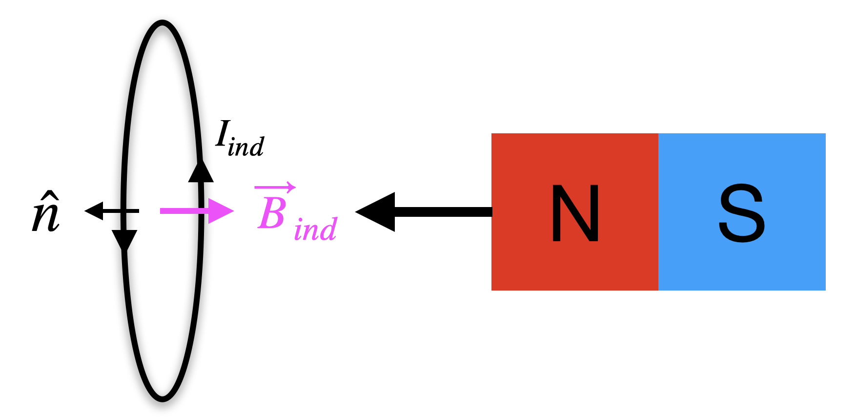
The area enclosed by the circuit is constant. The angle between the normal to the area of the circle loop and the field is constant, \(\theta=0\) and not changing. The magnitude of the magnetic field, \(|\vec B|\), field increases with time. Therefore, the changing magnetic field is the only contribution to the change in flux:

\[\frac{\Delta \Phi}{ \Delta t} =-A \frac{\Delta B}{ \Delta t}\]

We can turn the derivative in Equation \ref{flux} into just changes, "\(\Delta\)s", since we are assuming that the field is changing linearly with time. Since the magnitude increases linearly with time, the rate of change the magnetic field magnitude versus time is a constant: therefore the induced voltage will be constant.

The question we want tot answer is: will the current flow clockwise or counterclockwise? Now we use Lenz’s Law. To consider flux, let's choose the normal to be parallel to the magnetic field. In this example, since the magnetic field points from the north side of the magnet, this means that the normal vector will point to the left (as shown in the figure). This means the flux is positive and it increases with time. Based on Lenz's Law the induced current should oppose this. Thus, it will produce a negative magnetic flux through the loop that tries to cancel the increase in the positive flux. Since a positive flux means the field points to the left, then the magnetic field produced by the induced current, which we call the induced field, \(\vec B_{ind}\), will point to the right. Now can use the current right-hand-rule to established the direction of current based on the magnetic field,  \(\vec B_{ind}\), it produces. When you align your thumb along the tangent to the loop, and curl your fingers towards the induced magnetic field, your thumb will indicate the direction of the induced current. Since the induced field points to the right, we see that the induced current for this case is flowing in a counterclockwise direction as viewed from the right.

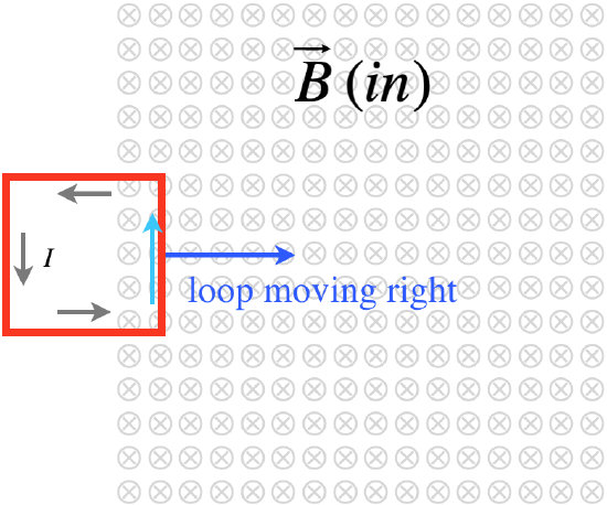
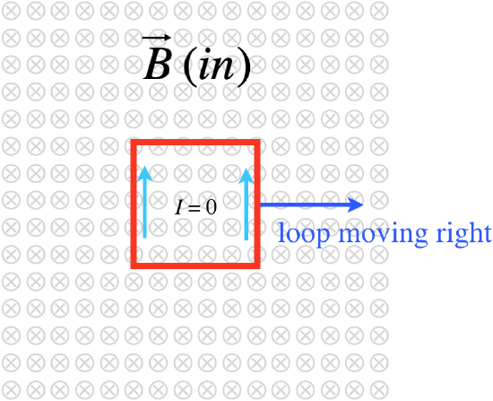
Below is another example of a conducting loop moving to the right into a uniform field which points into the page. Initially, there is no field through the loop. As it enters the field there is a flux into the page. To oppose this change the induced field will be out of the page. According to the right-hand-rule, this implies that the induced current will be counterclockwise as shown.

Figure 11.9.3: Conducting Loop Enters Uniform Magnetic Field

Next, as the loop continues to move to the right within the field, there is no longer a change in flux, this results in zero induced field and thus no current will flow.

Figure 11.9.4: Conducting Loop Stays Within the Uniform Magnetic Field

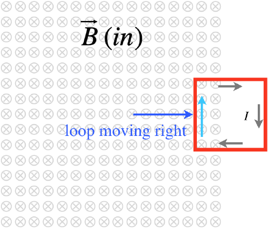
Finally, as the loop starts to exit the magnetic field, the flux that points into the page starts to decrease. To oppose this change, the induced flux and thus field will point into the page. With the help of the right-hand-rule we find that this must result in a clockwise induced current.

Figure 11.9.5: Conducting Loop Exits the Uniform Magnetic Field

We can explore directly how the changing flux is related to current by making a plot of flux as a function of time, as depicted in the figure below. Flux will always be into the page for this scenario since the magnetic field points into the page. If we will define the normal vector to point out of the page, the flux will be negative since the angle between flux and the normal vector is 180^o in this example. We also assume that flux changes linearly as the loop moves to the right at a constant speed. The flux starts at zero and its magnitude increases as the loop moves into the field. Since the flux is negative, this means that it becomes more negative. The constant flux region in the plot represent the part of the motion when the loop is fully immersed in the field, thus, the amount of flux does not change as it moves through it. As it starts exiting the field, the magnitude of flux starts to decrease or become less negative until it reaches zero when it fully exists the field.

Figure 11.9.6: Flux and Current as a Function of Time

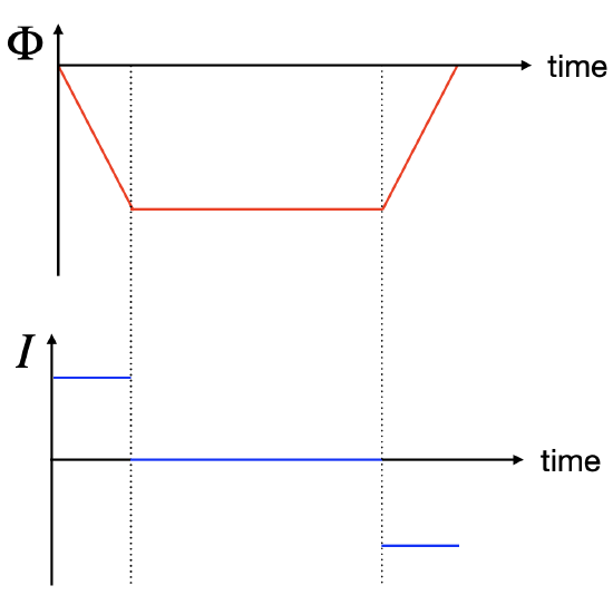
The plot also shows the induced current as a function of time. Equation \ref{Faraday} tells us that the induced current is the negative of the derivative of flux as a function of time. Initially, since the slope of the flux is constant and negative, this results in a constant positive current. This means that by defining flux into the page as negative, the change in flux will be also negative, so the induced field that opposes this change has to be positive. This leads to a counterclockwise induced current which by convention is then defined as positive. In the region where the flux is constant, the slope is zero, resulting in zero induced current. When the flux starts to decrease (become less negative), the slope is positive, resulting in a negative (clockwise) current.

Applications

We started discussing Faraday’s law by considering moving a magnet near a loop of wire. We have found that this produces an induced current in the wire. This phenomenon has found many familiar applications in the modern world:

• Seismograph: One way to exploit Faraday’s Law is to attach a magnet to anything that moves and place it near a loop of wire; any movement or oscillation in the object can be detected as an induced current in the wire loop. In this way we can translate physical movements and oscillations into electrical impulses. In all devices of this kind, the movement or oscillation is measured between the position of a coil relative to a magnet, whose movement causes the current in the coil to vary, generating an electrical signal. For example, as the vibrations produced by an earthquake pass through a seismograph, a magnet's vibrations produce a current that can be amplified to drive a plotting pen. This is how the seismograph operates.
• Guitar Pickup: Les Paul, a pioneer musician of pop-jazz guitar, applied Faraday’s Law to the making of musical instruments and invented the first electric guitar. The “pickup” of an electric guitar consists of a permanent magnet with a coil of wire wrapped around it several times. The permanent magnet is placed very close to the metal guitar strings. The magnetic field of the permanent magnet causes a part of the metal string of the guitar to become magnetized. When one plucks the string, it vibrates, creating a changing magnetic flux through the coil of wire surrounding the permanent magnet. The coil “picks up” the vibrations that generate an induced current and sends the signal to an amplifier, to the pleasure of rock fans everywhere.
• Electric Generator: An electric generator is used to efficiently convert mechanical energy to electrical energy. The mechanical energy can be provided by any number of means, such as falling water (like in a hydroelectric generator), expanding steam (as in coal, oil, and nuclear power plants), or wind (as in wind turbine generators). In all cases, the principle is the same, the mechanical energy is used to move a conducting wire coil inside a magnetic field (usually by rotating the wire). In this case, the area of the coil is the constant, the magnitude of the field is constant, so the angle term in the equation for Faraday's law is responsible for the changing flux. This is caused by the change in the relative orientation between the magnetic field and the normal to the area of the coil. Consider the simple scenario where we rotate the coil with constant angular speed \(\omega\). The rotation angle is given by \(\theta = \omega t\), and the flux will be proportional to \(\cos \omega t\). Using calculus, the time rate of change of the flux will then be proportional to \(\omega \sin \omega t\). This means the induced current will oscillate sinusoidally. In other words, the current in the coil alternates in direction, flowing in one direction for half the cycle and flowing the other direction for the other half. This kind of generator is referred to as an alternating current generator, or simply an AC generator. The standard plugs you use to power all of your electrical appliances are all powered by an electric generator of this form.
• Electric Motor: Electric motors work in basically the reverse principle that operates electric generators: an alternating electric current causes an electromagnetic cylinder to periodically switch poles, which interacts with the field of an inlaid magnet to turn it. Some motors use electromagnets for both components, but the principle is the same. The stationary magnetic piece is called the stator and the magnetic piece that rotates is called that rotor
• Hybrid Cars: Regenerative breaking discussed above.

Example \(\PageIndex{1}\)

Below are 4 cases: the left panels show the initial and the right panels show the final configurations. The arrows indicate the direction and magnitude of the external magnetic field.  

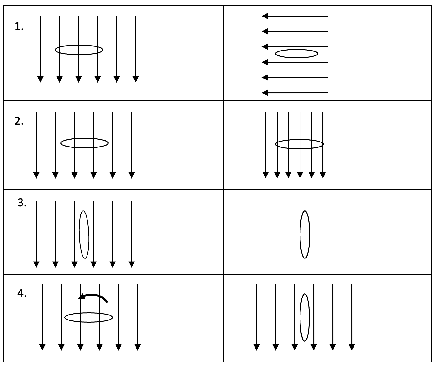
Fill in the table below for each case

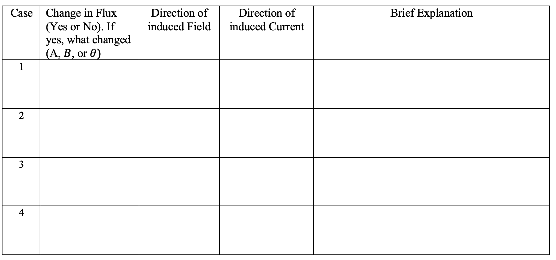
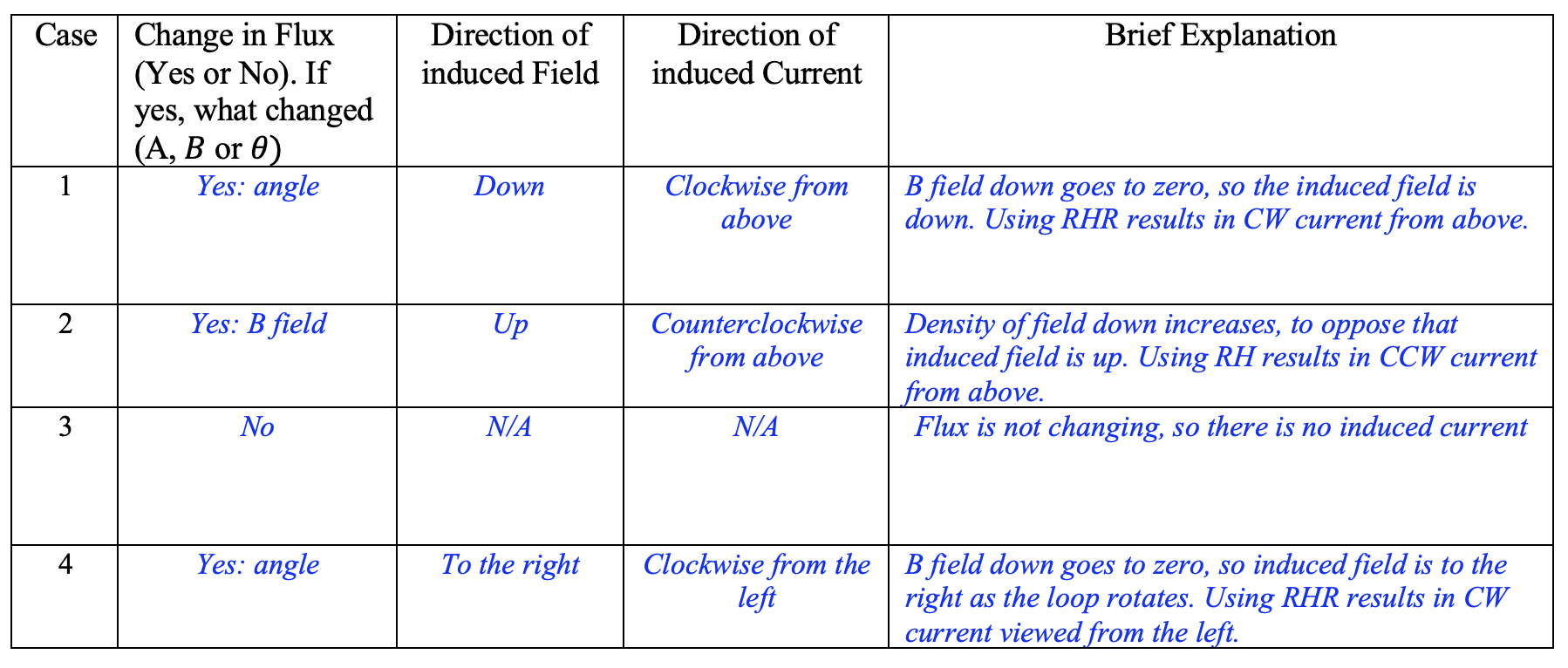
Solution

Example \(\PageIndex{2}\)

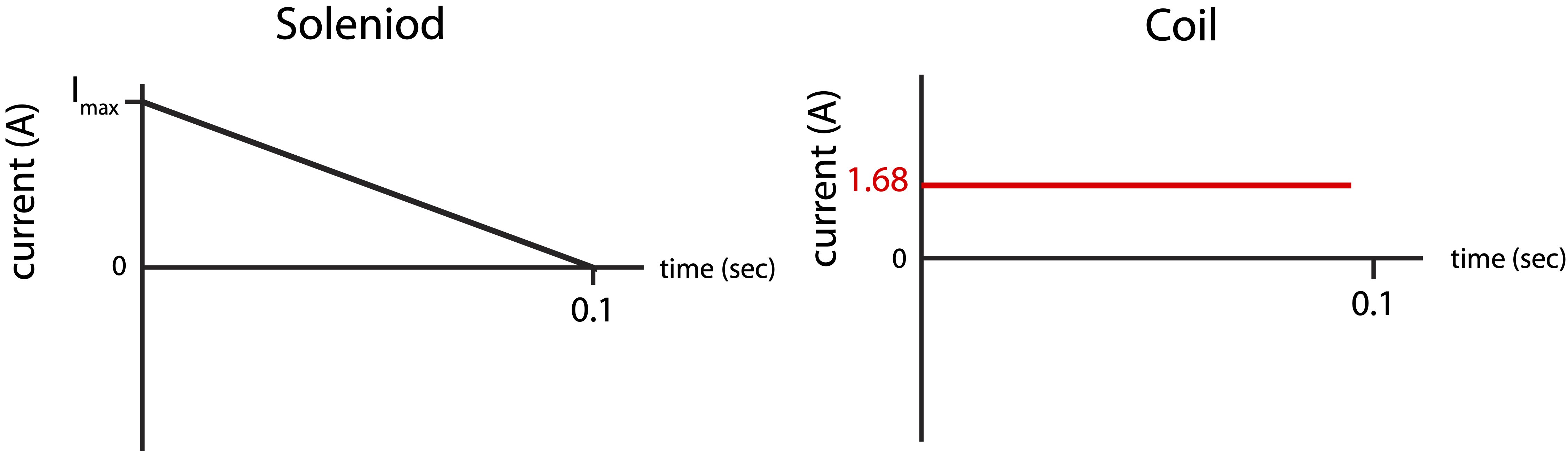
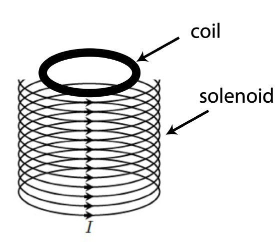
Consider a magnetic field is created by a large solenoid magnet. The solenoid is 1.5 meters long, has 5000 turns, a resistance of \(4\Omega\), and a one-meter radius. A coil located inside the solenoid has a single loop (as depicted below), a resistance of \(0.6\Omega\), and a 0.4 m radius. The solenoid initially has a current which produces a 0.2 T magnetic field. The solenoid’s current is then reduced linearly to zero in 0.1 seconds as shown in the left plot below.

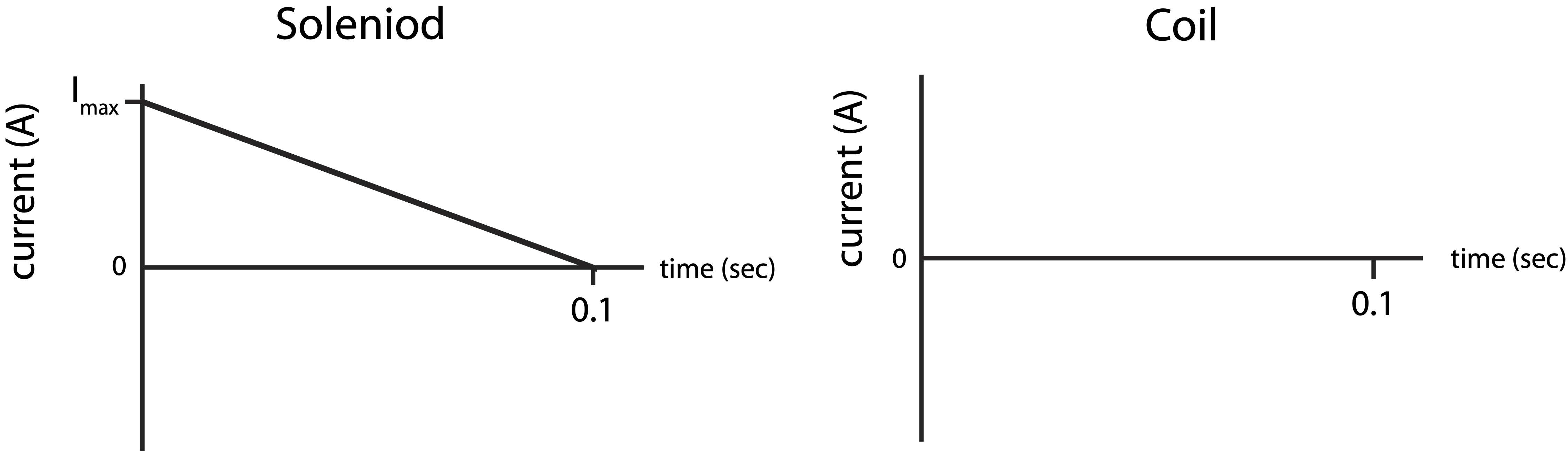
a) Calculate \(I_{max}\) which is marked on the plot below.

b) Make a graph of the current in the coil on the right plot below. Make sure to indicate numerical values and explain your choice of sign for the current.

Solution

a) The magnetic field for a solenoid is \(B=\dfrac{\mu_oIN}{L}\). The maximum current with be when the magnetic field is at 0.2 T, since the current is reduced with time:

\[I_{max}=\frac{BL}{\mu_oN}=\frac{0.2T\times1.5m}{4\times{10}^{-7}\frac{N}{A^2}\times5000}=47.7\ A\nonumber\]

b) The magnetic field is upward using the current RHR, which is reduced to zero. Thus, the induced magnetic field will also be upward to oppose the change of flux decreasing in the upward direction. Using the same RHR again, this results in an induced current which is counterclockwise as viewed from top. In other words, the direction of the current in the coil is the same as the direction of the current in the solenoid. 

Now that we have established the direction of current, we just need to worry about the magnitude of the induced emf and current. The magnitude of induced emf for the wire which only contains one loop is:

\[|\mathcal{E}|=\dfrac{d\Phi}{dt}=A\dfrac{\Delta B}{\Delta t}=\pi r^2\dfrac{dB}{dt}=(0.4^2\pi)m^2\dfrac{0.2T}{0.1s}=1.68A\nonumber\]

Solving for induced current:

\[I_{coil}=\dfrac{|\mathcal{E}|}{R}=\dfrac{1.0 V}{0.6\Omega}=1.68A\nonumber\]