2.1: Green’s Functions

I have spent so much time/space discussing the potential distributions created by a single point charge in various conductor geometries because for any of the geometries, the generalization of these results to the arbitrary distribution \(\ \rho(\mathbf{r})\) of free charges is straightforward. Namely, if a single charge \(\ q\), located at some point \(\ \mathbf{r}^{\prime}\), creates the electrostatic potential

\[\ \phi(\mathbf{r})=\frac{1}{4 \pi \varepsilon_{0}} q G\left(\mathbf{r}, \mathbf{r}^{\prime}\right),\tag{2.202}\]

then, due to the linear superposition principle, an arbitrary charge distribution (either discrete or continuous) creates the potential

Spatial Green’s function

\[\ \phi(\mathbf{r})=\frac{1}{4 \pi \varepsilon_{0}} \sum_{j} q_{j} G\left(\mathbf{r}, \mathbf{r}_{j}\right)=\frac{1}{4 \pi \varepsilon_{0}} \int \rho\left(\mathbf{r}^{\prime}\right) G\left(\mathbf{r}, \mathbf{r}^{\prime}\right) d^{3} r^{\prime}.\tag{2.203}\]

The function \(\ G\left(\mathbf{r}, \mathbf{r}^{\prime}\right)\) is called the (spatial) Green’s function – the notion very fruitful and hence popular in all fields of physics.⁶⁵ Evidently, as Eq. (1.35) shows, in the unlimited free space

\[\ G\left(\mathbf{r}, \mathbf{r}^{\prime}\right)=\frac{1}{\left|\mathbf{r}-\mathbf{r}^{\prime}\right|},\tag{2.204}\]

i.e. the Green’s function depends only on one scalar argument – the distance between the field-observation point \(\ \mathbf{r}\) and the field-source (charge) point \(\ \mathbf{r}^{\prime}\). However, as soon as there are conductors around, the situation changes. In this course, I will only discuss the Green’s functions that vanish as soon as the radius-vector \(\ \mathbf{r}\) points to the surface (S) of any conductor:⁶⁶

\[\ \left.G\left(\mathbf{r}, \mathbf{r}^{\prime}\right)\right|_{\mathbf{r} \in S}=0.\tag{2.205}\]

With this definition, it is straightforward to deduce the Green’s functions for the solutions of the last section’s problems in which conductors were grounded \(\ (\phi=0)\). For example, for a semi-space \(\ z \geq 0\) limited by a conducting plane \(\ z=0\) (Fig. 26), Eq. (185) yields

\[\ G=\frac{1}{\left|\mathbf{r}-\mathbf{r}^{\prime}\right|}-\frac{1}{\left|\mathbf{r}-\mathbf{r}^{\prime \prime}\right|}, \quad \text { with } \rho^{\prime \prime}=\rho^{\prime} \text { and } z^{\prime \prime}=-z^{\prime}.\tag{2.206}\]

We see that in the presence of conductors (and, as we will see later, any other polarizable media), the Green’s function may depend not only on the difference \(\ \mathbf{r}-\mathbf{r}^{’}\), but on each of these two arguments in a specific way.

So far, this looks just like re-naming our old results. The really non-trivial result of this formalism for electrostatics is that, somewhat counter-intuitively, the knowledge of the Green’s function for a system with grounded conductors (Fig. 30a) enables the calculation of the field created by voltage- biased conductors (Fig. 30b), with the same geometry. To show this, let us use the so-called Green’s theorem of the vector calculus.⁶⁷ The theorem states that for any two scalar, differentiable functions \(\ f(\mathbf{r})\) and \(\ g(\mathbf{r})\), and any volume \(\ V\),

\[\ \int_{V}\left(f \nabla^{2} g-g \nabla^{2} f\right) d^{3} r=\oint_{S}(f \nabla g-g \nabla f)_{n} d^{2} r,\tag{2.207}\]

where \(\ S\) is the surface limiting the volume. Applying the theorem to the electrostatic potential \(\ \phi(\mathbf{r})\) and the Green’s function \(\ G\) (also considered as a function of \(\ \mathbf{r}\)), let us use the Poisson equation (1.41) to replace \(\ \nabla^{2} \phi\) with \(\ \left(-\rho / \varepsilon_{0}\right)\), and notice that \(\ G\), considered as a function of \(\ \mathbf{r}\), obeys the Poisson equation with the \(\ \delta\)-functional source:

\[\ \nabla^{2} G\left(\mathbf{r}, \mathbf{r}^{\prime}\right)=-4 \pi \delta\left(\mathbf{r}-\mathbf{r}^{\prime}\right).\tag{2.208}\]

(Indeed, according to its definition (202), this function may be formally considered as the field of a point charge \(\ q=4 \pi \varepsilon_{0}\).) Now swapping the notation of the radius-vectors, \(\ \mathbf{r} \leftrightarrow \mathbf{r}’\), and using the Green’s function symmetry, \(\ G\left(\mathbf{r}, \mathbf{r}^{\prime}\right)=G\left(\mathbf{r}^{\prime}, \mathbf{r}\right)\),⁶⁸ we get

\[\ -4 \pi \phi(\mathbf{r})-\int_{V}\left(-\frac{\rho\left(\mathbf{r}^{\prime}\right)}{\varepsilon_{0}}\right) G\left(\mathbf{r}, \mathbf{r}^{\prime}\right) d^{3} r^{\prime}=\oint_{S}\left[\phi\left(\mathbf{r}^{\prime}\right) \frac{\partial G\left(\mathbf{r}, \mathbf{r}^{\prime}\right)}{\partial n^{\prime}}-G\left(\mathbf{r}, \mathbf{r}^{\prime}\right) \frac{\partial \phi\left(\mathbf{r}^{\prime}\right)}{\partial n^{\prime}}\right] d^{2} r^{\prime}.\tag{2.209}\]

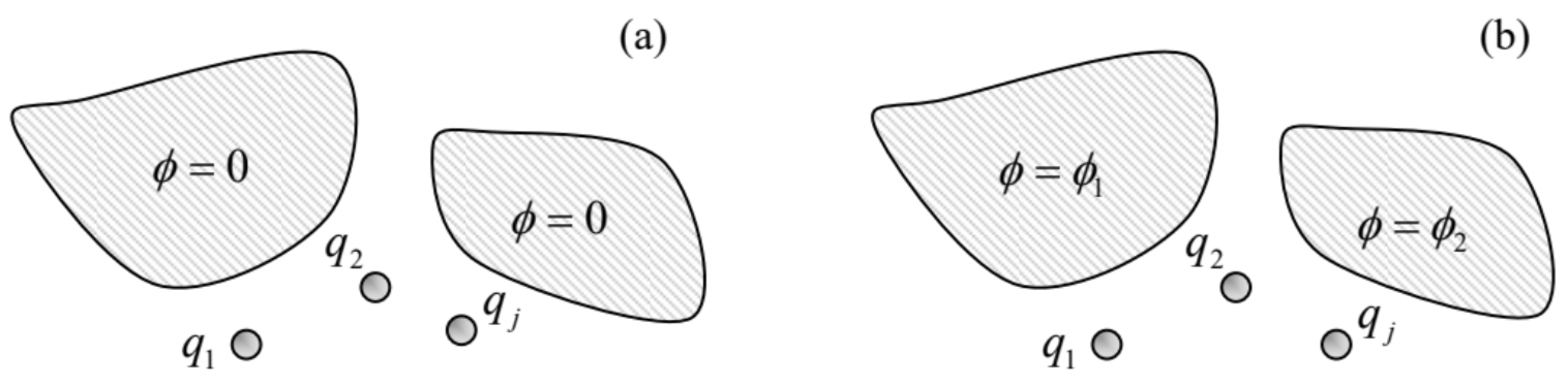Fig. 2.30. Green’s function method allows the solution of a simpler boundary problem (a) to be used to find the solution of a more complex problem (b), for the same conductor geometry.

Let us apply this relation to the volume \(\ V\) of free space between the conductors, and the boundary S drawn immediately outside of their surfaces. In this case, by its definition, Green’s function \(\ G\left(\mathbf{r}, \mathbf{r}^{\prime}\right)\) vanishes at the conductor surface \(\ (\mathbf{r} \in S)\) – see Eq. (205). Now changing the sign of \(\ \partial n^{\prime}\) (so that it would be the outer normal for conductors, rather than free space volume \(\ V\)), dividing all terms by \(\ 4 \pi\), and partitioning the total surface \(\ S\) into the parts (numbered by index j) corresponding to different conductors (possibly, kept at different potentials \(\ \phi_{k}\)), we finally arrive at the famous result:⁶⁹

Potential via Green’s function

\[\ \phi(\mathbf{r})=\frac{1}{4 \pi \varepsilon_{0}} \int_{V} \rho\left(\mathbf{r}^{\prime}\right) G\left(\mathbf{r}, \mathbf{r}^{\prime}\right) d^{3} r^{\prime}+\frac{1}{4 \pi} \sum_{k} \phi_{k} \oint_{S_{k}} \frac{\partial G\left(\mathbf{r}, \mathbf{r}^{\prime}\right)}{\partial n^{\prime}} d^{2} r^{\prime}.\tag{2.210}\]

While the first term on the right-hand side of this relation is a direct and evident expression of the superposition principle, given by Eq. (203), the second term is highly non trivial: it describes the effect of conductors with non-zero potentials \(\ \phi_{k}\) (Fig. 30b), using the Green’s function calculated for the
similar system with grounded conductors, i.e. with all \(\ \phi_{k}=0\) (Fig. 30a). Let me emphasize that since our volume \(\ V\) excludes conductors, the first term on the right-hand side of Eq. (210) includes only the stand-alone charges in the system (in Fig. 30, marked \(\ q_{1}\), \(\ q_{2}\), etc.), but not the surface charges of the conductors – which are taken into account, implicitly, by the second term.

In order to illustrate what a powerful tool Eq. (210) is, let us use to calculate the electrostatic field in two systems. In the first of them, a plane, circular, conducting disk, separated with a very thin cut from the remaining conducting plane, is biased with potential \(\ \phi=V\), while the rest of the plane is grounded – see Fig. 31.

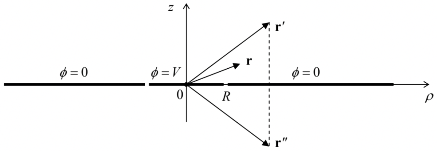Fig. 2.31. A voltage-biased conducting disk separated from the rest of a conducting plane.

If the width of the gap between the disk and the rest of the plane is negligible, we may apply Eq. (210) without stand-alone charges, \(\ \rho\left(\mathbf{r}^{\prime}\right)=0\), and the Green’s function for the uncut plane – see Eq. (206).⁷⁰ In the cylindrical coordinates, with the origin at the disk’s center (Fig. 31), the function is

\[\ \begin{aligned}
G\left(\mathbf{r}, \mathbf{r}^{\prime}\right) &=\frac{1}{\left[\rho^{2}+\rho^{\prime 2}-2 \rho \rho^{\prime} \cos \left(\varphi-\varphi^{\prime}\right)+\left(z-z^{\prime}\right)^{2}\right]^{1 / 2}} \\
&-\frac{1}{\left[\rho^{2}+\rho^{\prime 2}-2 \rho \rho^{\prime} \cos \left(\varphi-\varphi^{\prime}\right)+\left(z+z^{\prime}\right)^{2}\right]^{1 / 2}} .
\end{aligned}\tag{2.211}\]

(The sum of the first three terms under each square root in Eq. (211) is just the squared distance between the horizontal projections \(\ \boldsymbol{\rho}\) and \(\ \boldsymbol{\rho^{\prime}}\) of the vectors \(\ \mathbf{r}\) and \(\ \mathbf{r}^{\prime}\) (or \(\ \mathbf{r}^{\prime \prime}\)) correspondingly, while the last terms are the squares of their vertical displacements.)

Now we can readily calculate the derivative participating in Eq. (210), for \(\ z \geq 0\):

\[\ \left.\frac{\partial G}{\partial n^{\prime}}\right|_{s}=\left.\frac{\partial G}{\partial z^{\prime}}\right|_{z^{\prime}=+0}=\frac{2 z}{\left(\rho^{2}+\rho^{\prime 2}-2 \rho \rho^{\prime} \cos \left(\varphi-\varphi^{\prime}\right)+z^{2}\right)^{3 / 2}}.\tag{2.212}\]

Due to the axial symmetry of the system, we may take \(\ \varphi\) for zero. With this, Eqs. (210) and (212) yield

\[\ \phi=\frac{V}{4 \pi} \oint_{S} \frac{\partial G\left(\mathbf{r}, \mathbf{r}^{\prime}\right)}{\partial n^{\prime}} d^{2} r^{\prime}=\frac{V z}{2 \pi} \int_{0}^{2 \pi} d \varphi^{\prime} \int_{0}^{R} \frac{\rho^{\prime} d \rho^{\prime}}{\left(\rho^{2}+\rho^{\prime 2}-2 \rho \rho^{\prime} \cos \varphi^{\prime}+z^{2}\right)^{3 / 2}}.\tag{2.213}\]

This integral is not overly pleasing, but may be readily worked out at least for points on the symmetry axis \(\ (\rho=0, z \geq 0)\):⁷¹

\[\ \phi=V z \int_{0}^{R} \frac{\rho^{\prime} d \rho^{\prime}}{\left(\rho^{\prime 2}+z^{2}\right)^{3 / 2}}=\frac{V}{2} \int_{0}^{R^{2} / z^{2}} \frac{d \xi}{(\xi+1)^{3 / 2}}=V\left[1-\frac{z}{\left(R^{2}+z^{2}\right)^{1 / 2}}\right]\tag{2.214}\]

This result shows that if \(\ z \rightarrow 0\), the potential tends to \(\ V\) (as it should), while at \(\ z \gg R\),

\[\ \phi \rightarrow V \frac{R^{2}}{2 z^{2}}.\tag{2.215}\]

Now let us use the same Eq. (210) to solve the (in :-)famous problem of the cut sphere (Fig. 32). Again, if the gap between the two conducting semi-spheres is very thin \(\ (t<<R)\), we may use Green’s function for the grounded (and uncut) sphere. For a particular case \(\ \mathbf{r}^{\prime}=d \mathbf{n}_{z}\), this function is given by
Eqs. (197)-(198); generalizing the former relation for an arbitrary direction of vector \(\ \mathbf{r}’\), we get

\[\ G=\frac{1}{\left[r^{2}+r^{\prime 2}-2 r r^{\prime} \cos \gamma\right]^{1 / 2}}-\frac{R / r^{\prime}}{\left[r^{2}+\left(R^{2} / r^{\prime}\right)^{2}-2 r\left(R^{2} / r^{\prime}\right) \cos \gamma\right]^{1 / 2}}, \quad \text { for } r, r^{\prime} \geq R,\tag{2.216}\]

where \(\ \gamma\) is the angle between the vectors \(\ \mathbf{r}\) and \(\ \mathbf{r}’\), and hence \(\ \mathbf{r}^{\prime \prime}\) – see Fig. 32.

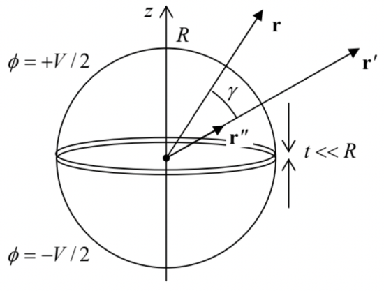Fig. 2.32. A system of two separated, oppositely biased semi-spheres.

Now, calculating the Green’s function’s derivative,

\[\ \left.\frac{\partial G}{\partial r^{\prime}}\right|_{r^{\prime}=R+0}=-\frac{\left(r^{2}-R^{2}\right)}{R\left[r^{2}+R^{2}-2 R r \cos \gamma\right]^{3 / 2}},\tag{2.217}\]

and plugging it into Eq. (210), we see that the integration is again easy only for the field on the symmetry axis (\(\ \mathbf{r}=z \mathbf{n}_{z}, \gamma=\theta\)), giving:

\[\ \phi=\frac{V}{2}\left[1-\frac{z^{2}-R^{2}}{z\left(z^{2}+R^{2}\right)^{1 / 2}}\right].\tag{2.218}\]

For \(\ z \rightarrow R\), this relation yields \(\ \phi \rightarrow V / 2\) (just checking :-), while for \(\ z / R \rightarrow \infty\),

\[\ \phi \rightarrow \frac{3 R^{2}}{4 z^{2}} V.\tag{2.219}\]

As will be discussed in the next chapter, such a field is typical for an electric dipole.

---

Reference

⁶⁵ See, e.g., CM Sec. 5.1, QM Secs. 2.2 and 7.4, and SM Sec. 5.5.

⁶⁶ \(\ G\) so defined is sometimes called the Dirichlet function.

⁶⁷ See, e.g., MA Eq. (12.3). Actually, this theorem is a ready corollary of the better-known divergence ("Gauss") theorem, MA Eq. (12.2).

⁶⁸ This symmetry, evident for the particular cases (204) and (206), may be readily proved for the general case by applying Eq. (207) to functions \(\ f(\mathbf{r}) \equiv G\left(\mathbf{r}, \mathbf{r}^{\prime}\right)\) and \(\ g(\mathbf{r}) \equiv G\left(\mathbf{r}, \mathbf{r}^{\prime \prime}\right)\). With this substitution, the left-hand side of that equality becomes equal to \(\ -4 \pi\left[G\left(\mathbf{r}^{\prime \prime}, \mathbf{r}^{\prime}\right)-G\left(\mathbf{r}^{\prime}, \mathbf{r}^{\prime \prime}\right)\right]\), while the right-hand side is zero, due to Eq. (205).

⁶⁹ In some textbooks, the sign before the surface integral is negative, because their authors use the outer normal to the free-space region V rather than that occupied by conductors – as I do.

⁷⁰ Indeed, if all parts of the cut plane are grounded, a narrow cut does not change the field distribution, and hence the Green’s function, significantly.

⁷¹ There is no need to repeat the calculation for \(\ z \leq 0\): from the symmetry of the problem, \(\ \phi(-z)=\phi(z)\).