2.2: Numerical Approach

Despite the richness of analytical methods, for many boundary problems (especially in geometries without a high degree of symmetry), the numerical approach is the only way to the solution. Though software packages offering their automatic numerical solution are abundant nowadays,⁷² it is important for every educated physicist to understand “what is under their hood”, at least because most universal programs exhibit mediocre performance in comparison with custom codes written for particular problems, and sometimes do not converge at all, especially for fast-changing (say, exponential) functions. The very brief discussion presented here⁷³ is a (hopefully, useful) fast glance under the hood, though it is certainly insufficient for professional numerical research work.

The simplest of the numerical approaches to the solution of partial differential equations, such as the Poisson or the Laplace equations (1.41)-(1.42), is the finite-difference method,⁷⁴ in which the sought continuous scalar function \(\ f(\boldsymbol{r})\), such as the potential \(\ \phi(\mathbf{r})\), is represented by its values in discrete points
of a rectangular grid (frequently called mesh) of the corresponding dimensionality – see Fig. 33.

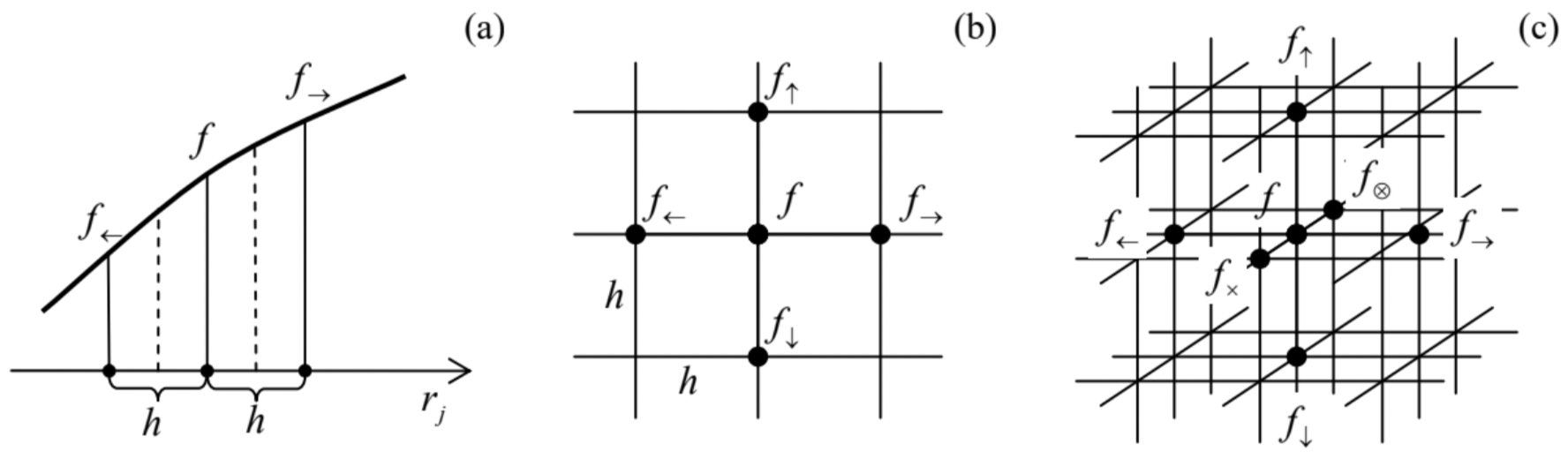Fig. 2.33. The general idea of the finite-difference method in (a) one, (b) two, and (c) three dimensions.

Each partial second derivative of the function is approximated by the formula that readily follows from the linear approximations of the function f and then its partial derivatives – see Fig. 33a:

\[\ \frac{\partial^{2} f}{\partial r_{j}^{2}} \equiv \frac{\partial}{\partial r_{j}}\left(\frac{\partial f}{\partial r_{j}}\right) \approx \frac{1}{h}\left(\left.\frac{\partial f}{\partial r_{j}}\right|_{r_{j}+h / 2}-\left.\frac{\partial f}{\partial r_{j}}\right|_{r_{j}-h / 2}\right) \approx \frac{1}{h}\left[\frac{f_{\rightarrow}-f}{h}-\frac{f-f_{\leftarrow}}{h}\right]=\frac{f_{\rightarrow}+f_{\leftarrow}-2 f}{h^{2}},\tag{2.220}\]

where \(\ f_{\rightarrow} \equiv f\left(r_{j}+h\right)\) and \(\ f_{\leftarrow} \equiv f\left(r_{j}-h\right)\). (The relative error of this approximation is of the order of \(\ h^{4} \partial^{4} f / \partial r_{j}^{4}\).) As a result, the action of a 2D Laplace operator on the function \(\ f\) may be approximated as

\[\ \frac{\partial^{2} f}{\partial x^{2}}+\frac{\partial^{2} f}{\partial y^{2}} \approx \frac{f_{\rightarrow}+f_{\leftarrow}-2 f}{h^{2}}+\frac{f_{\uparrow}+f_{\downarrow}-2 f}{h^{2}}=\frac{f_{\rightarrow}+f_{\leftarrow}+f_{\uparrow}+f_{\downarrow}-4 f}{h^{2}},\tag{2.221}\]

and of the 3D operator, as

\[\ \frac{\partial^{2} f}{\partial x^{2}}+\frac{\partial^{2} f}{\partial y^{2}}+\frac{\partial^{2} f}{\partial z^{2}} \approx \frac{f_{\rightarrow}+f_{\leftarrow}+f_{\uparrow}+f_{\downarrow}+f_{\otimes}+f_{\times}-6 f}{h^{2}}.\tag{2.222}\]

(The notation used in Eqs. (221)-(222) should be clear from Figs. 33b and 33c, respectively.)

As a simple example, let us apply this scheme to find the electrostatic potential distribution inside a cylindrical box with conducting walls and square cross-section \(\ a \times a\), using an extremely coarse mesh with step \(\ h=a / 2\) (Fig. 34). In this case, our function, the electrostatic potential \(\ \phi(x, y)\), equals zero at the side and bottom walls, and \(\ V_{0}\) at the top lid, so that, according to Eq. (221), the 2D Laplace equation may be approximated as

\[\ \frac{0+0+V_{0}+0-4 \phi}{(a / 2)^{2}}=0.\tag{2.223}\]

The resulting value for the potential in the center of the box is \(\ \phi=V_{0} / 4\).

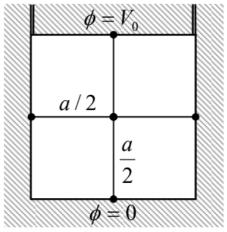Fig. 2.34. Numerically solving an internal 2D boundary problem for a conducting, cylindrical box with a square cross-section, using a very coarse mesh (with \(\ h=a / 2\)).

Surprisingly, this is the exact value! This may be proved by solving this problem by the variable separation method, just as this has been done for a similar 3D problem in Sec. 5. The result is

\[\ \phi(x, y)=\sum_{n=1}^{\infty} c_{n} \sin \frac{\pi n x}{a} \sinh \frac{\pi n y}{a}, \quad c_{n}=\frac{4 V_{0}}{\pi n \sinh (\pi n)} \times\left\{\begin{array}{l}
1, \text { if } n \text { is odd,} \\
0, \text { otherwise.}
\end{array}\right.\tag{2.224}\]

so that at the central point \(\ (x=y=a / 2)\),

\[\ \phi=\frac{4 V_{0}}{\pi} \sum_{j=0}^{\infty} \frac{\sin [\pi(2 j+1) / 2] \sinh [\pi(2 j+1) / 2]}{(2 j+1) \sinh [\pi(2 j+1)]} \equiv \frac{2 V_{0}}{\pi} \sum_{j=0}^{\infty} \frac{(-1)^{j}}{(2 j+1) \cosh [\pi(2 j+1) / 2]}.\tag{2.225}\]

The last series equals exactly to \(\ \pi / 8\), so that \(\ \phi=V_{0} / 4\).⁷⁵

so that \(\ \phi=V_{0} / 6\). Unbelievably enough, this result is also exact! (This follows from our variable separation result expressed by Eqs. (95) and (99) with \(\ a = b = c\).)

Though such exact results should be considered as a happy coincidence rather than the general law, they still show that numerical methods, even with relatively crude meshes, may be more computationally efficient than the “analytical” approaches, like the variable separation method with its infinite-sum results that, in most cases, require computers anyway – at least for the result’s comprehension and analysis.

A more powerful (but also much more complex) approach is the finite-element method in which the discrete point mesh, typically with triangular cells, is (automatically) generated in accordance with the system geometry.⁷⁶ Such mesh generators provide higher point concentration near sharp convex parts of conductor surfaces, where the field concentrates and hence the potential changes faster, and thus ensure better accuracy-to-speed trade-off than the finite-difference methods on a uniform grid. The price to pay for this improvement is the algorithm’s complexity that makes manual adjustments much harder. Unfortunately, in this series, I do not have time for going into the details of that method and have to refer the reader to the special literature on this subject.⁷⁷

---

Reference

⁷² See, for example, MA Secs. 16 (iii) and (iv).

⁷³ It is almost similar to that given in CM Sec. 8.5 and is reproduced here for the reader’s convenience, being illustrated with examples from this (EM) course.

⁷⁴ For more details see, e.g., R. Leveque, Finite Difference Methods for Ordinary and Partial Differential Equations, SIAM, 2007.

⁷⁵ Let me leave it for the reader to derive this result from Eq. (210) and the system’s symmetry, without any calculations.

⁷⁶ See, e.g., CM Fig. 8.14.

⁷⁷ See, e.g., either C. Johnson, Numerical Solution of Partial Differential Equations by the Finite Element Method, Dover, 2009, or T. Hughes, The Finite Element Method, Dover, 2000.