2.3: Exercise Problems

Exercise 2.1

Calculate the force (per unit area) exerted on a conducting surface by an external electric field, normal to it. Compare the result with the electric field’s definition given by Eq. (1.6), and comment.

Exercise 2.2

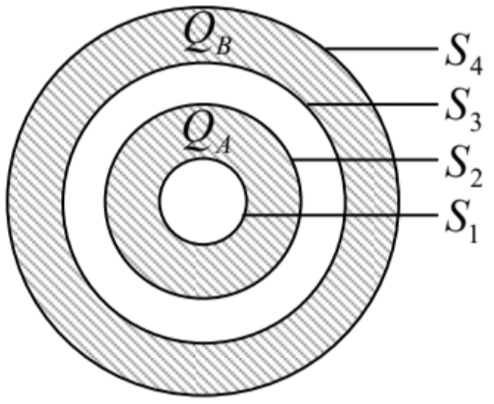
Electric charges \(\ Q_{A}\) and \(\ Q_{B}\) have been placed on two metallic, concentric spherical shells – see the figure on the right. What is the full charge of each of the surfaces \(\ S_{1}-S_{4}\)?

Exercise 2.3

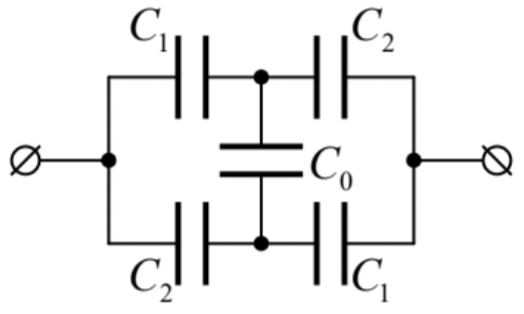
Calculate the mutual capacitance between the terminals of the lumped-capacitor circuit shown in the figure on the right. Analyze and interpret the result for major particular cases.

Exercise 2.4

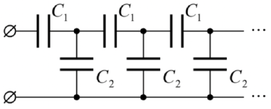
Calculate the mutual capacitance between the terminals of the semi-infinite lumped-capacitor circuit shown in the figure on the right, and the law of decay of the applied voltage along the system.

Exercise 2.5

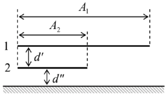
A system of two thin conducting plates is located over a ground plane as shown in the figure on the right, where \(\ A_{1}\) and \(\ A_{2}\) are the areas of the indicated plate parts, while \(\ d^{\prime}\) and \(\ d^{\prime \prime}\) are the distances between them. Neglecting the fringe effects, calculate:

(i) the effective capacitance of each plate, and

(ii) their mutual capacitance.

Exercise 2.6

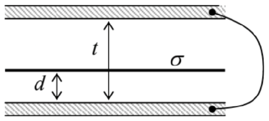
A wide, thin plane film, carrying a uniform electric charge density \(\ \sigma\), is placed inside a plane capacitor whose plates are connected with a wire (see the figure on the right), and were initially electroneutral. Neglecting the edge effects, calculate the surface charges of the plates, and the net force acting upon the film (per unit area).

Exercise 2.7

Following up on the discussion of two weakly coupled spheres in Sec. 2, find an approximate expression for the mutual capacitance (per unit length) between two very thin, parallel wires, both with round cross-sections, but each with its own radius. Compare the result with that for two small spheres, and interpret the difference.

Exercise 2.8

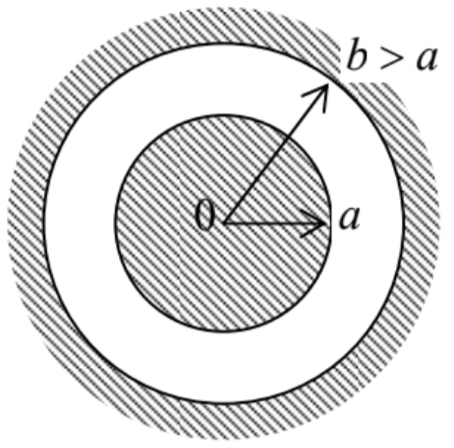
Use the Gauss law to calculate the mutual capacitance of the following two-electrode systems, with the cross-section shown in Fig. 7 (reproduced on the right):

(i) a conducting sphere inside a concentric spherical cavity in another conductor, and

(ii) a long conducting cylinder inside a coaxial cavity in another conductor, i.e. a coaxial cable. (In this case, we speak about the capacitance per unit length).

Compare the results with those obtained in Sec. 2.2 using the Laplace equation solution.

Exercise 2.9

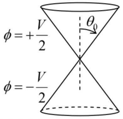
Calculate the electrostatic potential distribution around two barely separated conductors in the form of coaxial, round cones (see the figure on the right), with voltage \(\ V\) between them. Compare the result with that of a similar 2D problem, with the cones replaced by plane-face wedges. Can you calculate the mutual capacitances between the conductors in these systems? If not, can you estimate them?

Exercise 2.10

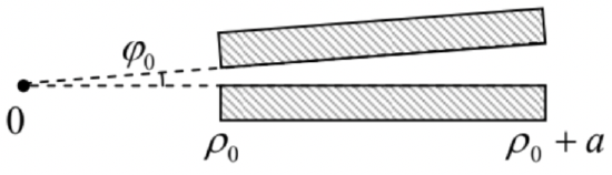
Calculate the mutual capacitance between two rectangular, plane electrodes of area \(\ A=a \times l\), with a small angle \(\ \varphi_{0}<<a / \rho_{0}\) between them – see the figure on the right.

Exercise 2.11

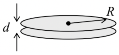
Using the results for a single thin round disk, obtained in Sec. 4, consider a system of two such disks at a small distance \(\ d<<R\) from each other –
see the figure on the right. In particular, calculate:

(i) the reciprocal capacitance matrix of the system,

(ii) the mutual capacitance between the disks,

(iii) the partial capacitance, and

(iv) the effective capacitance of one disk,

(all in the first nonzero approximation in \(\ d / R<<1\)). Compare the results (ii)-(iv) and interpret their
similarities and differences.

Exercise 2.12^*

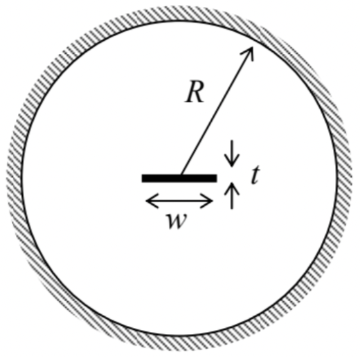
Calculate the mutual capacitance (per unit length) between two cylindrical conductors forming a system with the cross-section shown in the figure on the right, in the limit \(\ t<<w<<R\).

Hint: You may like to use elliptical (not “ellipsoidal”!) coordinates \(\ \{\alpha, \beta\}\) defined by the following equality:

\(\ x+i y=c \cosh (\alpha+i \beta),(*)\)

with the appropriate choice of the constant \(\ c\). In these orthogonal 2D coordinates, the Laplace operator is very simple:⁷⁸

\(\ \nabla^{2}=\frac{1}{c^{2}\left(\cosh ^{2} \alpha-\cos ^{2} \beta\right)}\left(\frac{\partial^{2}}{\partial \alpha^{2}}+\frac{\partial^{2}}{\partial \beta^{2}}\right).\)

Exercise 2.13

Formulate 2D electrostatic problems that can be solved using each of the following analytic functions of the complex variable \(\ \boldsymbol{z} \equiv x+i y\):

(i) \(\ \boldsymbol{w}=\ln \boldsymbol{z},\)

(ii) \(\ \boldsymbol{w}=\boldsymbol{z}^{1 / 2},\)

and solve these problems.

Exercise 2.14

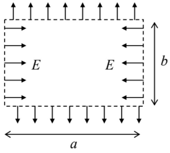
On each side of a cylindrical volume with a rectangular cross-section \(\ a \times b\), with no electric charges inside it, the electric field is uniform, normal to the side’s plane, and opposite to that on the opposite side – see the figure on the right. Calculate the distribution of the electric potential inside the volume, provided that the field’s magnitude on the vertical sides equals \(\ E\). Suggest a practicable method to implement such potential distribution.

Exercise 2.15

Complete the solution of the problem shown in Fig. 12, by calculating the distribution of the surface charge of the semi-planes. Can you calculate the mutual capacitance between the plates (per unit length)? If not, can you estimate it?

Exercise 2.16^*

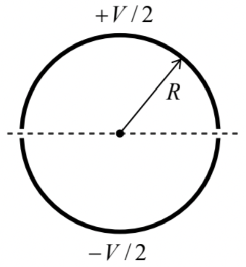
A straight, long, thin, round-cylindrical metallic pipe has been cut, along its axis, into two equal parts – see the figure on the right.

(i) Use the conformal mapping method to calculate the distributions of the electrostatic potential, created by voltage \(\ V\) applied between the two parts, both outside and inside the pipe, and of the surface charge.

(ii) Calculate the mutual capacitance between pipe’s halves (per unit length), taking into account a small width \(\ 2 t<<R\) of the cut.

Hints: In Task (i), you may like to use the following complex function:

\(\ \boldsymbol{w}=\ln \left(\frac{R+\boldsymbol{z}}{R-\boldsymbol{z}}\right),\)

while in Task (ii), it is advisable to use the solution of the previous problem.

Exercise 2.17

Solve Task (i) of the previous problem using the variable separation method, and compare the results.

Exercise 2.18

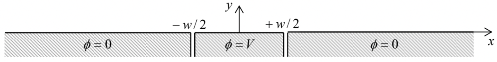
Use the variable separation method to calculate the potential distribution above the plane surface of a conductor, with a strip of width w separated by very thin cuts, and biased with voltage \(\ V\) – see the figure below.

Exercise 2.19

The previous problem is now modified: the cut-out and voltage-biased part of the conducting plane is now not a strip, but a square with side w. Calculate the potential distribution above the conductor’s surface.

Exercise 2.20

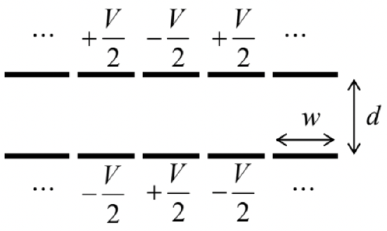
Each electrode of a large plane capacitor is cut into long strips of equal width w, with very narrow gaps between them. These strips are kept at alternating potentials, as shown in the figure on the right. Use the variable separation method to calculate the electrostatic potential distribution in space, and explore the limit \(\ w<<d\).

Exercise 2.21

Complete the cylinder problem started in Sec. 7 (see Fig. 17), for the cases when the top lid’s voltage is fixed as follows:

(i) \(\ V=V_{0} J_{1}\left(\xi_{11} \rho / R\right) \sin \varphi\), where \(\ \xi_{11} \approx 3.832\) is the first root of the Bessel function \(\ J_{1}(\xi)\);

(ii) \(\ V=V_{0}=\text { const }\).

For both cases, calculate the electric field at the centers of the lower and upper lids. (For Task (ii), an answer including series and/or integrals is acceptable.)

Exercise 2.22

For an infinitely long system sketched in Fig. 21:

(i) calculate and sketch the distribution of the electrostatic potential inside the system for various values of the ratio \(\ R / h\), and

(ii) simplify the results for the limit \(\ R / h \rightarrow 0\).

Exercise 2.23

Use the variable separation method to find the potential distribution inside and outside of a thin spherical shell of radius \(\ R\), with a fixed potential distribution: \(\ \phi(R, \theta, \varphi)=V_{0} \sin \theta \cos \varphi\).

Exercise 2.24

A thin spherical shell carries an electric charge with areal density \(\ \sigma=\sigma_{0} \cos \theta\). Calculate the spatial distribution of the electrostatic potential and the electric field, both inside and outside the shell.

Exercise 2.25

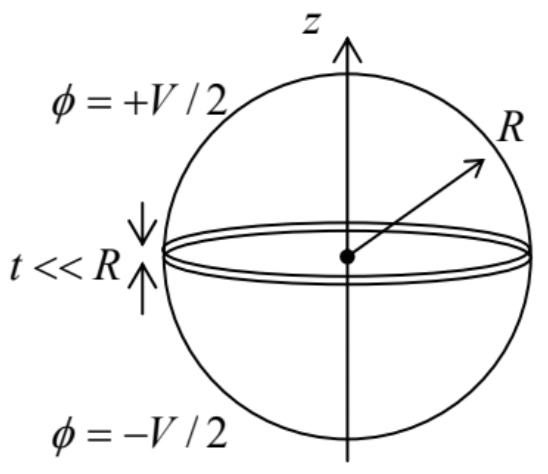
Use the variable separation method to calculate the potential distribution both inside and outside of a thin spherical shell of radius \(\ R\), separated with a very thin cut, along the central plane \(\ z=0\), into two halves, with voltage \(\ V\) applied between them – see the figure on the right.

Analyze the solution; in particular, compare the field at the axis \(\ z\), for \(\ z>R\), with Eq. (218).

Hint: You may like to use the following integral of a Legendre polynomial with odd index \(\ l=1,3,5 \ldots=2 n-1\):⁷⁹

\(\ I_{n} \equiv \int_{0}^{1} P_{2 n-1}(\xi) d \xi=\frac{1}{n !} \cdot\left(\frac{1}{2}\right) \cdot\left(-\frac{3}{2}\right) \cdot\left(-\frac{5}{2}\right) \ldots\left(\frac{3}{2}-n\right) \equiv(-1)^{n-1} \frac{(2 n-3) ! !}{2 n(2 n-2) ! !}.\)

Exercise 2.26

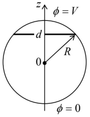
Calculate, up to the terms \(\ O\left(1 / r^{2}\right)\), the long-range electric field induced by a split and voltage-biased conducting sphere – similar to that discussed in Sec. 7 (see Fig. 32) and in the previous problem, but with the cut’s plane at an arbitrary distance \(\ d<R\) from the center – see the figure on the right.

Exercise 2.27

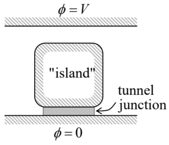
A small conductor (in this context, usually called the single-electron island) is placed between two conducting electrodes, with voltage V applied between them. The gap between the island and one of the electrodes is so narrow that electrons may tunnel quantum-mechanically through this “junction” – see the figure on the right. Neglecting thermal excitations, calculate the equilibrium charge of the island as a function of \(\ V\).

Hint: To solve this problem, you do not need to know much about the quantum-mechanical tunneling between conductors, besides that such tunneling of an electron, followed by energy relaxation of the resulting excitations, may be considered as a single inelastic (energy-dissipating) event. At negligible thermal excitations, such an event takes place only when it decreases the total potential energy of the system.⁸⁰

Exercise 2.28

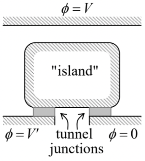
The system discussed in the previous problem is now generalized as the figure on the right shows. If the voltage \(\ V^{\prime}\) applied between the two bottom electrodes is sufficiently large, electrons can successively tunnel through two junctions of this system (called the single-electron transistor), carrying dc current between these electrodes. Neglecting thermal excitations, calculate the region of voltages \(\ V\) and \(\ V^{\prime}\) where such a current is fully suppressed (Coulomb-blocked).

Exercise 2.29

Use the image charge method to calculate the full surface charges induced in the plates of a very broad, voltage-unbiased plane capacitor of thickness \(\ D\) by a point charge \(\ q\) separated from one of the electrodes by distance \(\ d\).

Exercise 2.30

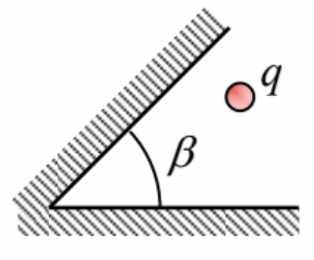
Prove the statement, made in Sec. 9, that the 2D boundary problem shown in the figure on the right, can be solved using a finite number of image charges if the angle \(\ \beta\) equals \(\ \pi / n\), where \(\ n=1,2, \ldots\)

Exercise 2.31

Use the image charge method to calculate the potential energy of the electrostatic interaction between a point charge placed in the center of a spherical cavity that had been carved inside a grounded conductor, and the cavity’s walls. Looking at the result, could it be obtained in a simpler way (or ways)?

Exercise 2.32

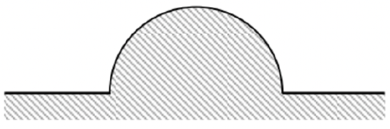
Use the method of images to find the Green’s function of the system shown in the figure on the right, where the bulge on the conducting plane has the shape of a semi-sphere of radius \(\ R\).

Exercise 2.33^*

Use the spherical inversion, expressed by Eq. (198), to develop an iterative method for a more and more precise calculation of the mutual capacitance between two similar metallic spheres of radius \(\ R\), with centers separated by distance \(\ d>2 R\).

Exercise 2.34^*

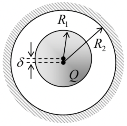
A metallic sphere of radius \(\ R_{1}\), carrying electric charge \(\ Q\), is placed inside a spherical cavity of radius \(\ R_{2}>R_{1}\), carved inside another metal.
Calculate the electric force exerted on the sphere if its center is displaced by a small distance \(\ \delta<<R_{1}, R_{2}-R_{1}\) from that of the cavity – see the figure on the right.

Exercise 2.35

Within the simple models of the electric field screening in conductors, discussed in Sec. 2.1, analyze the partial screening of the electric field of a point charge \(\ q\) by a plane, uniform conducting film of thickness \(\ t<<\lambda\), where \(\ \lambda\) is (depending on charge carrier statistics) either the Debye or the Thomas-Fermi screening length – see, respectively, Eqs. (8) or (10). Assume that the distance \(\ d\) between the charge and the film is much larger than \(\ t\).

Exercise 2.36

Suggest a convenient definition of the Green’s function for 2D electrostatic problems, and calculate it for:

(i) the unlimited free space, and

(ii) the free space above a conducting plane.

Use the latter result to re-solve Problem 18.

Exercise 2.37

Calculate the 2D Green’s functions for the free spaces:

(i) outside a round conducting cylinder, and

(ii) inside a round cylindrical hole in a conductor.

Exercise 2.38

Solve Task (i) of Problem 16 (see also Problem 17), using Green’s function method.

Exercise 2.39

Solve the 2D boundary problem that was discussed in Sec. 11 (Fig. 34) using:

(i) the finite difference method, with a finer square mesh, \(\ h=a / 3\), and

(ii) the variable separation method.

Compare the results at the mesh points, and comment.

---

Reference

⁷⁹ As a reminder, the double factorial (also called “semifactorial”) operator (!!) is similar to the usual factorial operator (!), but with the product limited to numbers of the same parity as its argument – in our particular case, of the odd numbers in the numerator, and even numbers in the denominator.

⁸⁰ Strictly speaking, this model, implying negligible quantum-mechanical coherence of the tunneling events, is correct only if the junction transparency is sufficiently low, so that its effective electric resistance is much higher than the quantum unit of resistance (see, e.g., QM Sec. 3.2), \(\ R_{\mathrm{Q}} \equiv \pi \hbar / 2 e^{2} \approx 6.5 \mathrm{k} \Omega\) – which may be readily done in experiment.