3.5: Electric Field Energy in a Dielectric

In Chapter 1, we have obtained two key results for the electrostatic energy: Eq. (1.55) for a charge interaction with an independent (“external”) field, and a similarly structured formula (1.60), but with an additional factor 1⁄2, for the field induced by the charges under consideration. These relations are universal, i.e. valid for dielectrics as well, provided that the charge density includes all charges (including those bound into the elementary dipoles). However, it is convenient to recast them into a form depending on the density \(\ \rho(\mathbf{r})\) of only stand-alone charges.

If a field is created only by stand-alone charges under consideration and is proportional to \(\ \rho(\mathbf{r})\) (requiring that we deal with linear dielectrics only), we can repeat all the argumentation of the beginning of Sec. 1.3, and again arrive at Eq. (1.60), provided that \(\ \phi\) is now the macroscopic field’s potential. Now we can recast this result in the terms of fields – essentially as this was done in Eqs. (1.62)-(1.64), but now making a clear difference between the macroscopic electric field \(\ \mathbf{E}=-\nabla \phi\) and the electric displacement field D that obeys the macroscopic Maxwell equation (32). Plugging \(\ \rho(\mathbf{r})\), expressed from that equation, into Eq. (1.60), we get

\[\ U=\frac{1}{2} \int(\nabla \cdot \mathbf{D}) \phi d^{3} r.\tag{3.69}\]

Using the fact²⁷ that for differentiable functions \(\ \phi\) and D,

\[\ (\nabla \cdot \mathbf{D}) \phi=\nabla \cdot(\phi \mathbf{D})-(\nabla \phi) \cdot \mathbf{D},\tag{3.70}\]

we may rewrite Eq. (69) as

\[\ U=\frac{1}{2} \int \nabla \cdot(\phi \mathbf{D}) d^{3} r-\frac{1}{2} \int(\nabla \phi) \cdot \mathbf{D} d^{3} r.\tag{3.71}\]

The divergence theorem, applied to the first term on the right-hand side, reduces it to a surface integral of \(\ \phi D_{n}\). (As a reminder, in Eq. (1.63) the integral was of \(\ \phi(\nabla \phi)_{n} \propto \phi E_{n}\).) If the surface of the volume we are considering is sufficiently far, this surface integral vanishes. On the other hand, the gradient in the second term of Eq. (71) is just (minus) field E, so that it gives

\[\ U=\frac{1}{2} \int \mathbf{E} \cdot \mathbf{D} d^{3} r=\frac{1}{2} \int E(\mathbf{r}) \varepsilon(\mathbf{r}) E(\mathbf{r}) d^{3} r \equiv \frac{\varepsilon_{0}}{2} \int \kappa(\mathbf{r}) E^{2}(\mathbf{r}) d^{3} r.\quad\quad\quad\text{Field energy in a linear dielectric}\tag{3.73}\]

\[\ U=\frac{1}{2} \int \mathbf{E} \cdot \mathbf{D} d^{3} r=\frac{1}{2} \int E(\mathbf{r}) \varepsilon(\mathbf{r}) E(\mathbf{r}) d^{3} r \equiv \frac{\varepsilon_{0}}{2} \int \kappa(\mathbf{r}) E^{2}(\mathbf{r}) d^{3} r.\tag{3.72}\]

This expression is a natural generalization of Eq. (1.65), and shows that we can, as we did in free space, represent the electrostatic energy in a local form:²⁸

\[\ U=\int u(\mathbf{r}) d^{3} r, \quad \text { with } u=\frac{1}{2} \mathbf{E} \cdot \mathbf{D}=\frac{\varepsilon}{2} E^{2}=\frac{D^{2}}{2 \varepsilon} .\quad\quad\quad\quad\text{Field energy in a linear dielectric} \tag{3.73}\]

As a sanity check, in the trivial case \(\ \varepsilon=\varepsilon_{0}(\text { i.e. } \kappa=1)\), this result is reduced to Eq. (1.65).

Of course, Eq. (73) is valid only for linear dielectrics, because our starting point, Eq. (1.60), is only valid if \(\ \phi\) is proportional to \(\ \rho\). To make our calculation more general, we should intercept the calculations of Sec. 1.3 at an earlier stage, at which we have not yet used this proportionality. For example, the first of Eqs. (1.56) may be rewritten, in the continuous limit, as

\[\ \delta U=\int \phi(\mathbf{r}) \delta \rho(\mathbf{r}) d^{3} r,\tag{3.74}\]

where the symbol \(\ \delta\) means a small variation of the function – e.g., its change in time, sufficiently slow to ignore the relativistic and magnetic-field effects. Applying such variation to Eq. (32), and plugging the resulting relation \(\ \delta \rho=\nabla \cdot \delta \mathbf{D}\) into Eq. (74), we get

\[\ delta U=\int(\nabla \cdot \delta \mathbf{D}) \phi d^{3} r.\tag{3.75}\]

(Note that in contrast to Eq. (69), this expression does not have the front factor 1⁄2.) Now repeating the same calculations as in the linear case, for the energy density variation we get a remarkably simple (and general!) expression,

\[\ \delta u=\mathbf{E} \cdot \delta \mathbf{D} \equiv \sum_{j=1}^{3} E_{j} \delta D_{j}, \quad\quad\quad\quad\text{Energy density’s variation}\tag{3.76}\]

where the last expression uses the Cartesian components of the vectors \(\ \mathbf{E}\) and \(\ \mathbf{D}\). This is as far as we can go for the general dependence \(\ \mathbf{D}(\mathbf{E})\). If the dependence is linear and isotropic, as in Eq. (46), then \(\ \delta\mathbf{D}=\varepsilon \delta \mathbf{E}\) and

\[\ \delta u=\varepsilon \mathbf{E} \cdot \delta \mathbf{E} \equiv \varepsilon \delta\left(\frac{E^{2}}{2}\right).\tag{3.77}\]

The integration of this expression over the whole variation, from the field equal to zero to a certain final distribution \(\ \mathbf{E}(\mathbf{r})\), brings us back to Eq. (73).

An important role of Eq. (76), in its last form, is to indicate that the Cartesian coordinates of \(\ \mathbf{E}\) may be interpreted as generalized forces, and those of \(\ \mathbf{D}\) as generalized coordinates of the field’s effect on a unit volume of the dielectric. This allows one, in particular, to form the proper Gibbs potential energy²⁹ of a system with an electric field \(\ \mathbf{E}(\mathbf{r})\) fixed, at every point, by some external source:

\[\ \text{Gibbs potential energy}\quad\quad\quad\quad U_{\mathrm{G}}=\int_{V} u_{\mathrm{G}}(\mathbf{r}) d^{3} r, \quad u_{\mathrm{G}}(\mathbf{r})=u(\mathbf{r})-\mathbf{E}(\mathbf{r}) \cdot \mathbf{D}(\mathbf{r}).\tag{3.78}\]

The essence of this notion is that if the generalized external force (in our case, \(\ \mathbf{E}\)) is fixed, the stable equilibrium of the system corresponds to the minimum of \(\ U_{\mathrm{G}}\), rather than of the potential energy \(\ U\) as such – in our case, that of the field in our system.

As the simplest illustration of this concept, let us consider a very long cylinder (with an arbitrary cross-section’s shape), made of a uniform linear dielectric, placed into a uniform external electric field, parallel to the cylinder’s axis – see Fig. 13.

Fig. 3.13. A cylindrical dielectric sample in a longitudinal external electric field.

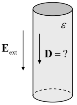
For this simple problem, the equilibrium value of \(\ \mathbf{D}\) inside the cylinder may be, of course, readily found without any appeal to energies. Indeed, the solution of the Laplace equation inside the cylinder, with the boundary condition (37) is evident: \(\ \mathbf{E}(\mathbf{r})=\mathbf{E}_{\mathrm{ext}}\), and so that Eq. (46) immediately yields \(\ \mathbf{D}_{\mathbf{(r)}}=\varepsilon \mathbf{E}_{\mathrm{ext}}\). However, one may wonder why does the minimum of the potential energy \(\ U\), given by Eq. (73) in its last form,

\[\ \frac{U}{V}=\frac{D^{2}}{2 \varepsilon},\tag{3.79}\]

correspond to a different (zero) value of \(\ \mathbf{D}\). The Gibbs potential energy (78) immediately removes the contradiction. Indeed, for our uniform case, this energy per unit volume of the cylinder is

\[\ \frac{U_{\mathrm{G}}}{V}=\frac{U}{V}-\mathbf{E} \cdot \mathbf{D}=\frac{D^{2}}{2 \varepsilon}-\mathbf{E} \cdot \mathbf{D} \equiv \sum_{j=1}^{3}\left(\frac{D_{j}^{2}}{2 \varepsilon}-E_{j} D_{j}\right),\tag{3.80}\]

and its minimum as a function of every Cartesian component of \(\ \mathbf{D}\) corresponds to the correct value of the displacement: \(\ D_{j}=\varepsilon E_{j}\), i.e. \(\ \mathbf{D}=\varepsilon \mathbf{E}=\varepsilon \mathbf{E}_{\text {ext }}\). So, the minimum of the Gibbs potential energy indeed corresponds to the systems’ equilibrium, and it may be very useful for analyses of the polarization dynamics.

Note also that Eq. (80), at this equilibrium point (only!), may be rewritten as

\[\ \frac{U_{\mathrm{G}}}{V}=\frac{U}{V}-\mathbf{E} \cdot \mathbf{D}=\frac{D^{2}}{2 \varepsilon}-\frac{\mathbf{D}}{\varepsilon} \cdot \mathbf{D} \equiv-\frac{D^{2}}{2 \varepsilon},\tag{3.81}\]

i.e. formally coincides with Eq. (79), besides the opposite sign. Another useful general relation (not limited to linear dielectrics) may be obtained by taking the variation of the uG expressed by Eq. (78), and then using Eq. (76):

\[\ \delta u_{\mathrm{G}}=\delta u-\delta(\mathbf{E} \cdot \mathbf{D})=\mathbf{E} \cdot \delta \mathbf{D}-(\delta \mathbf{E} \cdot \mathbf{D}+\mathbf{E} \cdot \delta \mathbf{D}) \equiv-\mathbf{D} \cdot \delta \mathbf{E} .\tag{3.82}\]

In order to see how these expressions (with their perhaps counter-intuitive negative signs³⁰) work, let us plug \(\ mathbf{D}\) from Eq. (33):

\[\ \delta u_{\mathrm{G}}=-\left(\varepsilon_{0} \mathbf{E}+\mathbf{P}\right) \cdot \delta \mathbf{E} \equiv-\delta\left(\frac{\varepsilon_{0} E^{2}}{2}\right)-\mathbf{P} \cdot \delta \mathbf{E} .\tag{3.83}\]

So far, this relation is general. In the particular case when the polarization \(\ \mathbf{P}\) is field-independent, we may integrate Eq. (83) over the full electric field’s variation, say from 0 to some finite value \(\ \mathbf{E}\), getting

\[\ u_{\mathrm{G}}=-\frac{\varepsilon_{0} E^{2}}{2}-\mathbf{P} \cdot \mathbf{E}.\tag{3.84}\]

Again, the Gibbs energy is relevant only if \(\ \mathbf{E}\) is dominated by an external field \(\ \mathbf{E}_{\mathrm{ext}}\), independent of the orientation of the polarization \(\ \mathbf{P}\). If, in addition, \(\ \mathbf{P}(\mathbf{r}) \neq 0\) only in some finite volume \(\ V\), we may integrate Eq. (84) over the volume, getting

\[\ U_{\mathrm{G}}=-\mathbf{p} \cdot \mathbf{E}_{\text {ext }}+\text { const, } \quad \text { with } \mathbf{p} \equiv \int_{V} \mathbf{P}(\mathbf{r}) d^{3} r,\tag{3.85}\]

where “const” means the terms independent of \(\ \mathbf{p}\). In this expression, we may readily recognize Eq. (15a) for an electric dipole \(\ \mathbf{p}\) of a fixed magnitude, which was obtained in Sec. 1 in a different way.

This comparison shows again that \(\ U_{\mathrm{G}}\) is nothing extraordinary; it is just the relevant part of the potential energy of the system in a fixed external field, including the energy of its interaction with the field. Still, I would strongly recommend the reader to get a better gut feeling of the relation between the two potential energies, \(\ U\) and \(\ U_{\mathrm{G}}\) – for example, by using them to solve a very simple problem: calculate the force of attraction between the plates of a plane capacitor.

---

Reference

²⁷ See, e.g., MA Eq. (11.4a).

²⁸ In the Gaussian units, each of the last three expressions should be divided by \(\ 4 \pi\).

²⁹ See, e.g., CM Sec. 1.4, in particular Eq. (1.41), and Sec. 2.1. Note that as Eq. (78) clearly illustrates, once again, that the difference between the potnetial energies \(\ U_{\mathrm{G}}\) and \(\ U\), usually discussed in courses of statistical physics and/or thermodynamics as the difference between the Gibbs and Helmholtz free energies (see, e.g., SM 1.4), is more general than the effects of random thermal motion, addressed by these disciplines.

³⁰ Some psychological relief may be provided that the fact that you may add to \(\ U_{\mathrm{G}}\) (and \(\ U\)) any constant – positive if you like.