
7.7: Dielectric Waveguides, Optical Fibers, and Paraxial Beams


- Last updated
- Mar 5, 2022
- Save as PDF

( \newcommand{\kernel}{\mathrm{null}\,}\)
Now let us discuss electromagnetic wave propagation in dielectric waveguides. The simplest, step-index waveguide (see Figs. 23b and 25) consists of an inner core and an outer shell (in the optical fiber technology lingo, called cladding) with a higher wave propagation speed, i.e. a lower index of refraction:
ν+>ν−, i.e. n+<n−,k+<k−,ε+μ+<ε−μ−.
at the same frequency. (In most cases the difference is achieved due to that in the electric permittivity, ε+<ε−, while magnetically both materials are virtually passive: μ−≈μ+≈μ0, so that their refraction indices n±, defined by Eq. (84), are very close to (ε±/ε0)1/2; I will limit my discussion to this approximation.)
The basic idea of waveguide’s operation may be readily understood in the limit when the wavelength λ is much smaller than the characteristic size R of the core’s cross-section. In this “geometric optics” limit, at the distances of the order of λ from the core-to-cladding interface, which determines the wave reflection, we can neglect the interface’s curvature and approximate its geometry with a plane. As we know from Sec. 4, if the angle θ of the wave’s incidence on such an interface is larger than the critical value θc specified by Eq. (85), the wave is totally reflected. As a result, the waves launched into the fiber core at such “grazing” angles, propagate inside the core, being repeatedly reflected from the cladding – see Fig. 25.

The most important type of dielectric waveguides is optical fibers.59 Due to a heroic technological effort during three decades starting from the mid-1960s, the attenuation of such fibers has been decreased from the values of the order of 20 db/km (typical for a window glass) to the fantastically low values about 0.2 db/km (meaning virtually perfect transparency of 10-km-long fiber segments!), combined with the extremely low plane-wave (“chromatic”) dispersion below 10ps/km⋅nm.60 In conjunction with the development of inexpensive erbium-based quantum amplifiers, this breakthrough has enabled inter-city and inter-continental (undersea), broadband61 optical cables, which are the backbone of all the modern telecommunication infrastructure.
The only bad news is that these breakthroughs were achieved for just one kind of materials (silica-based glasses)62 within a very narrow range of their chemical composition. As a result, the dielectric constants κ±≡ε±/ε0 of the cladding and core of practical optical fibers are both close to 2.2 (n±≈1.5) and hence very close to each other, so that the relative difference of the refraction indices,
Δ≡n−−n+n−=ε1/2−−ε1/2+ε1/2−≈ε−−ε+2ε±
is typically below 0.5%. This factor limits the fiber bandwidth. Indeed, let us use the geometric-optics picture to calculate the number of quasi-plane-wave modes that may propagate in the fiber. For the complementary angle (Fig. 25)
ϑ≡π2−θ, so that sinθ=cosϑ
Eq. (85) gives the following propagation condition:
cosϑ>n+n−=1−Δ.
In the limit Δ<<1, when the incidence angles θ>θc of all propagating waves are very close to π/2, and hence the complementary angles are small, we can keep only two first terms in the Taylor expansion of the left-hand side of Eq. (151) and get
ϑ2max≈2Δ.
(Even for the higher-end value Δ=0.005, this critical angle is only ~0.1 radian, i.e. close to 5∘.) Due to this smallness, we may approximate the maximum transverse component of the wave vector as
(kt)max=k(sinϑ)max≈kϑmax≈√2kΔ,
and use Eq. (147) to calculate the number N of propagating modes:
N≈2(πR2)(πk2ϑ2max)(2π)2=(kR)2Δ.
For typical values k=0.73×10⁷ m−1 (corresponding to the free-space wavelength λ0=nλ=2πn/k≈1.3μm), R=25μm, and Δ=0.005, this formula gives N≈150.
Now we can calculate the geometric dispersion of such a fiber, i.e. the difference of the mode propagation speed, which is commonly characterized in terms of the difference between the wave delay times (traditionally measured in picoseconds per kilometer) of the fastest and slowest modes. Within the geometric optics approximation, the difference of time delays of the fastest mode (with kz=k) and the slowest mode (with kz=ksinθc) at distance l is
Δt=Δ(lνz)=Δ(kzlω)=lωΔkz=lν(1−sinθc)=lν(1−n+n−)≡lνΔ.
For the example considered above, the TEM wave’s speed in the glass, ν=c/n≈2×108 m/s, and the geometric dispersion Δt/l is close to 25ps/m, i.e. 25,000 ps/km. (This means, for example, that a 1-ns pulse, being distributed between the modes, would spread to a ~25-ns pulse after passing a just 1-km fiber segment.) This result should be compared with the chromatic dispersion mentioned above, below 10ps/km⋅nm, which gives dt/l is of the order of only 1,000 ps/km in the whole communication band dλ∼100 nm. Due to this high geometric dispersion, such relatively thick (2R∼50 nm) multi-mode fibers are used for the transfer of signals power over only short distances below ~ 100 m. (As compensation, they may carry relatively large power, beyond 10 mW.)
Long-range telecommunications are based on single-mode fibers, with thin cores (typically with diameters 2R∼5μm, i. e. of the order of λ/Δ1/2). For such structures, Eq. (154) yields N∼1, but in this case the geometric optics approximation is not quantitatively valid, and for the fiber analysis, we should get back to the Maxwell equations. In particular, this analysis should take into explicit account the evanescent wave in the cladding, because its penetration depth may be comparable with R.63
Since the cross-section of an optical fiber lacks metallic walls, the Maxwell equations describing them cannot be exactly satisfied with either TEM-wave, or H-mode, or E-mode solutions. Instead, the fibers can carry the so-called HE and EH modes, with both vectors H and E having longitudinal components simultaneously. In such modes, both Ez and Hz inside the core (ρ≤R) have a form similar to Eq. (141):
f−=flJn(ktρ)cosn(φ−φ0), where k2t=k2−−k2z>0, and k2−≡ω2ε−μ−,
where the constant angles φ0 may be different for each field. On the other hand, for the evanescent wave in the cladding, we may rewrite Eqs. (101) as
(∇2−κ2t)f+=0, where κ2t≡k2z−k2+>0, and k2+≡ω2ε+μ+.
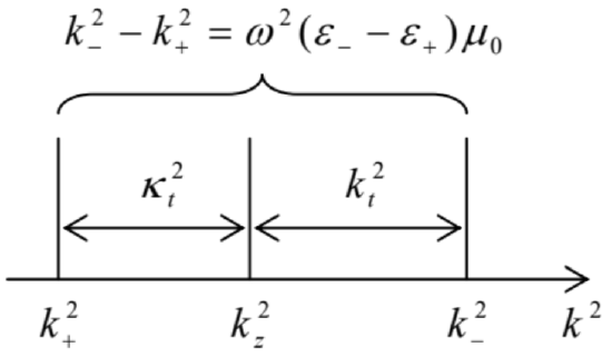
Figure 26 illustrates these relations between kt,κt,kz, and k±; note that the following sum,
k2t+κ2t=ω2(ε−−ε+)μ0=2k2Δ,Universal relation between kt and κt
is fixed (at a given frequency) and, for typical fibers, is very small (<<k2). In particular, Fig. 26 shows that neither kt nor κt can be larger than ω[(ε−−ε+)μ0]1/2=(2Δ)1/2k. This means that the depth δ=1/κt of the wave penetration into the cladding is at least 1/k(2Δ)1/2=λ/2π(2Δ)1/2>>λ/2π. This is why the cladding layers in practical optical fibers are made as thick as ∼50μm, so that only a negligibly small tail of this evanescent wave field reaches their outer surfaces.
In the polar coordinates, Eq. (157) becomes
[1ρ∂∂ρ(ρ∂∂ρ)+1ρ2∂2∂φ2−κ2t]f+=0,
- the equation to be compared with Eq. (139) for the circular metallic-wall waveguide. From Sec. 2.7 we know that the eigenfunctions of Eq. (159) are the products of the sine and cosine functions of nφ by a linear combination of the modified Bessel functions In and Kn shown in Fig. 2.22, now of the argument κtρ. The fields have to vanish at ρ→∞, so that only the latter functions (of the second kind) can participate in the solution:
f+∝Kn(κtρ)cosn(φ−φ0).
Now we have to reconcile Eqs. (156) and (160), using the boundary conditions at ρ=R for both longitudinal and transverse components of both fields, with the latter components first calculated using Eqs. (121). Such a conceptually simple, but a bit bulky calculation (which I am leaving for the reader’s exercise), yields a system of two linear, homogeneous equations for the complex amplitudes El and Hl, which are compatible if
(k2−ktJ′nJn+k2+κtK′nKn)(1ktJ′nJn+1κtK′nKn)=n2R2(k2−k2t+k2+κ2t)(1k2t+1κ2t),
where the prime signs (as a rare exception in this series) denote the derivatives of each function over its full argument: ktρ for Jn, and κtρ for Kn.
For any given frequency ω, the system of equations (158) and (161) determines the values of kt and κt, and hence kz. Actually, for any n>0, this system provides two different solutions: one corresponding to the so-called HE wave, with a larger ratio Ez/Hz, and the EH wave, with a smaller value of that ratio. For angular-symmetric modes with n=0 (for whom we might naively expect the lowest cutoff frequency), the equations may be satisfied by the fields having just one non-zero longitudinal component (either Ez or Hz), so that the HE modes are the usual E waves, while the EH modes are the H waves. For the H modes, the characteristic equation is reduced to the requirement that the expression in the second parentheses on the left-hand side of Eq. (161) is equal to zero. Using the Bessel function identities J′0=−J1 and K′0=−K1, this equation may be rewritten in a simpler form:
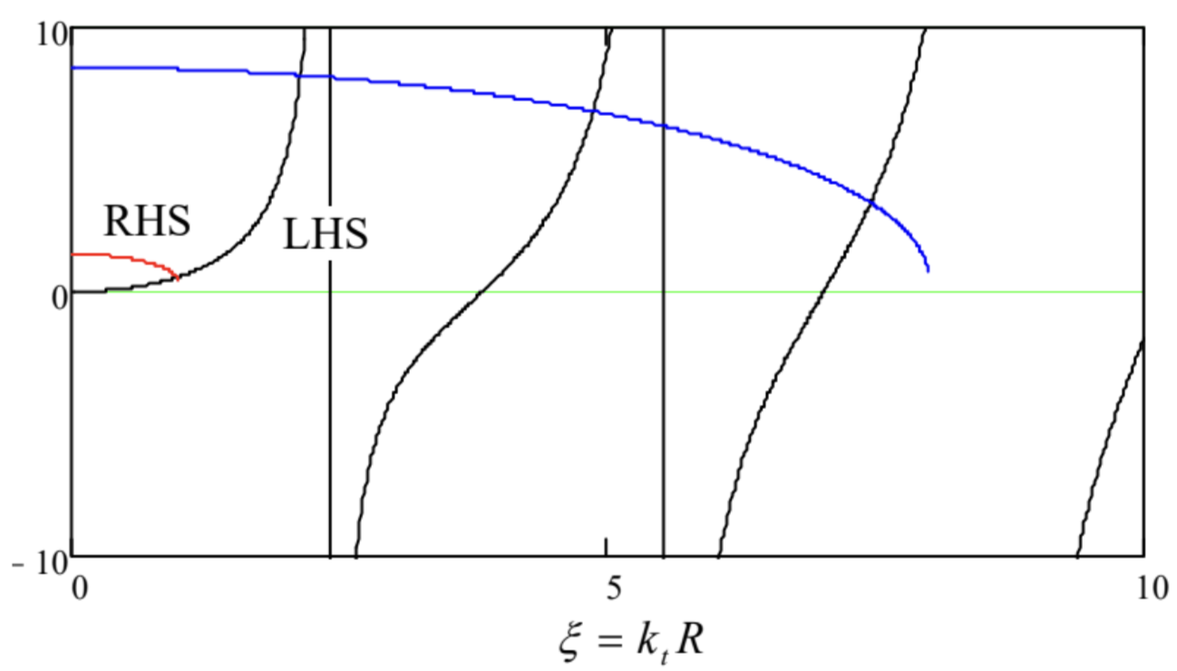
1ktJ1(ktR)J0(ktR)=−1κtK1(κtR)K0(κtR).
Using the universal relation between kt and κt given by Eq. (158), we may plot both sides of Eq. (162) as functions of the same argument, say, ξ≡ktR – see Fig. 27.

The right-hand side of Eq. (162) depends not only on ξ, but also on the dimensionless parameter V defined as the normalized right-hand side of Eq. (158):
V2≡ω2(ε−−ε+)μ0R2≈2Δk2±R2.
(According to Eq. (154), if V>>1, it gives twice the number N of the fiber modes – the conclusion confirmed by Fig. 27, taking into account that it describes only the H modes.) Since the ratio K1/K0 is positive for all values of the functions’ argument (see, e.g., the right panel of Fig. 2.22), the right-hand side of Eq. (162) is always negative, so that the equation may have solutions only in the intervals where the ratio J1/J0 is negative, i.e. at
ξ01<ktR<ξ11,ξ02<ktR<ξ12,…,
where ξnm is the m-th zero of the function Jn(ξ) – see Table 2.1. The right-hand side of the characteristic equation (162) diverges at κtR→0, i.e. at ktR→V, so that no solutions are possible if V is below the critical value Vc=ξ01≈2.405. At this cutoff point, Eq. (163) yields k±≈ξ01/R(2Δ)1/2. Hence, the cutoff frequency of the lowest H mode corresponds to the TEM wavelength
λmax=2πRξ01(2Δ)1/2≈3.7RΔ1/2.
For typical parameters Δ=0.005 and R=2.5μm, this result yields λmax∼0.65μm, corresponding to the free-space wavelength λ0∼1μm. A similar analysis of the first parentheses on the left-hand side of Eq. (161) shows that at Δ→0, the cutoff frequency for the E modes is similar.
This situation may look exactly like that in metallic-wall waveguides, with no waves possible at frequencies below ωc, but this is not so. The basic reason for the difference is that in the metallic waveguides, the approach to ωc results in the divergence of the longitudinal wavelength λz≡2π/kz. On the other hand, in dielectric waveguides, the approach leaves λz finite (kz→k+). Due to this difference, a certain linear superposition of HE and EH modes with n=1 can propagate at frequencies well below the cutoff frequency for n=0, which we have just calculated.64 This mode, in the limit ε+≈ε− (i.e. Δ<<1) allows a very interesting and simple description using the Cartesian (rather than polar) components of the fields, but still expressed as functions of the polar coordinates ρ and φ. The reason is that this mode is very close to a linearly polarized TEM wave. (Due to this reason, this mode is referred to as LP01.)
Let us select the x-axis parallel to the transverse component of the magnetic field vector at ρ=0, so that Ex|ρ=0=0, but Ey|ρ=0≠0, and Hx∣ρ=0≠0, but Hy∣ρ=0=0. The only suitable solutions of the 2D Helmholtz equation (that should be obeyed not only by the z-components of the field, but also their x- and y-components) are proportional to J0(ktρ), with zero coefficients for Ex and Hy.
Now we can use the last two equations of Eqs. (100) to calculate the longitudinal components of the fields:
Ez=1−ikz∂Ey∂y=−iktkzE0J1(ktρ)sinφ,Hz=1−ikz∂Hx∂x=−iktkzH0J1(ktρ)cosφ,
where I have used the following mathematical identities: J′0=−J1,∂ρ/∂x=x/ρ=cosφ, and ∂ρ/∂y=y/ρ=sinφ. As a sanity check, we see that the longitudinal component or each field is a (legitimate!) eigenfunction of the type (141), with n=1. Note also that if kt<<kz (this relation is always true if Δ<<1 – see either Eq. (158) or Fig. 26), the longitudinal components of the fields are much smaller than their transverse counterparts, so that the wave is indeed very close to the TEM one. Because of that, the ratio of the electric and magnetic field amplitudes is also close to that in the TEM wave: E0/H0≈Z−≈Z+.
Now to satisfy the boundary conditions at the core-to-cladding interface ( ρ=R), we need to have a similar angular dependence of these components at ρ≥R. The longitudinal components of the fields are tangential to the interface and thus should be continuous. Using the solutions similar to Eq. (160) with n=1, we get
Ez=−iktkzJ1(ktR)K1(κtR)E0K1(κtρ)sinφ,Hz=−iktkzJ1(ktR)K1(κtR)H0K1(κtρ)cosφ, for ρ≥R.
For the transverse components, we should require the continuity of the normal magnetic field μHn, for our simple field structure equal to just μHxcosφ, of the tangential electric field Eτ=Eysinφ, and of the normal component of Dn=εEn=εEycosφ. Assuming that μ−=μ+=μ0, and ε+≈ε−.65 we can satisfy these conditions with the following solutions:
Ex=0,Ey=J0(ktR)K0(κtR)E0K0(κtρ),Hx=J0(ktR)K0(ktR)H0K0(κtρ),Hy=0, for ρ≥R.
From here, we can calculate components from Ez and Hz, using the same approach as for ρ≤R:
Ez=1−ikz∂Ey∂y=−iκtkzJ0(ktR)K0(κtR)E0K1(κtρ)sinφ,Hz=1−ikz∂Hx∂x=−iκtkzJ0(ktR)K0(κtR)H0K1(κtρ)cosφ, for ρ≥R.
These relations provide the same functional dependence of the fields as Eqs. (167), i.e. the internal and external fields are compatible, but their amplitudes at the interface coincide only if
LP01 mode: characteristic equationktJ1(ktR)J0(ktR)=κtK1(κtR)K0(κtR).
This characteristic equation (which may be also derived from Eq. (161) with n=1 in the limit Δ→0) looks close to Eq. (162), but functionally is much different from it – see Fig. 28. Indeed, its right-hand side is always positive, and the left-hand side tends to zero at ktR→0. As a result, Eq. (171) may have a solution for arbitrary small values of the parameter V defined by Eq. (163), i.e. for arbitrary low frequencies (large wavelengths). This is why this mode is used in practical single-mode fibers: there are no other modes with wavelength larger than λmax given by Eq. (165), so that they cannot be unintentionally excited on small inhomogeneities of the fiber.
It is easy to use the Bessel function approximations by the first terms of the Taylor expansions (2.132) and (2.157) to show that in the limit V→0, κtR tends to zero much faster than ktR≈V:κtR→2exp{−1/V}<<V. This means that the scale ρc≡1/κt of the radial distribution of the LP01 wave’s fields in the cladding becomes very large. In this limit, this mode may be interpreted as a virtually TEM wave propagating in the cladding, just slightly deformed (and guided) by the fiber’s core. The drawback of this feature is that it requires very thick cladding, to avoid energy losses in its outer (“buffer” and “jacket”) layers that defend the silica layers from the elements, but lack their low optical absorption. Due to this reason, the core radius is usually selected so that the parameter V is just slightly less than the critical value Vc=ξ01≈2.4 for higher modes, thus ensuring the single-mode operation.
In order to reduce the field spread into the cladding, the step-index fibers discussed above may be replaced with graded-index fibers whose dielectric constant ε is gradually and slowly decreased from the center to the periphery.66 Keeping only the main two terms in the Taylor expansion of the function ε(ρ) at ρ=0, we may approximate such reduction as
ε(ρ)≈ε(0)(1−ζρ2),
where ζ≡−[(d2ε/dρ2)/2ε]ρ=0 is a positive constant characterizing the fiber composition gradient.67 Moreover, if this constant is sufficiently small (ζ<<k2), the field distribution across the fiber’s cross-section may be described by the same 2D Helmholtz equation (101), but with a space-dependent transverse wave vector:68
[∇2t+k2t(ρ)]f=0,wherek2t(ρ)=k2(ρ)−k2z≡k2t(0)−k2(0)ζρ2, and k2(0)≡ω2ε(0)μ0.
Surprisingly for such an axially-symmetric problem, because of its special dependence on the radius, this equation may be most readily solved in the Cartesian coordinates. Indeed, rewriting it as
[∂2∂x2+∂2∂y2+k2t(0)−k2(0)ζ(x2+y2)]f=0,
and separating the variables as f=X(x)Y(y), we get
1Xd2Xdx2+1Yd2Ydy2+k2t(0)−k2(0)ζ(x2+y2)=0,
so that the functions \ X and \ Y obey similar differential equations, for example
\ \frac{d^{2} X}{d x^{2}}+\left[k_{x}^{2}-k^{2}(0) \zeta x^{2}\right] X=0,\tag{7.176}
with the separation constants satisfying the following condition:
\ k_{x}^{2}+k_{y}^{2}=k_{t}^{2}(0) \equiv k^{2}(0)-k_{z}^{2}.\tag{7.177}
The ordinary differential equation (176) is well known from elementary quantum mechanics, because the stationary Schrödinger equation for one of the most important basic quantum systems, a 1D harmonic oscillator, may be rewritten in this form. Its eigenvalues are very simple:
\ \left(k_{x}^{2}\right)_{n}=k(0) \zeta^{1 / 2}(2 n+1), \quad\left(k_{y}^{2}\right)_{m}=k(0) \zeta^{1 / 2}(2 m+1), \quad \text { with } n, m=0,1,2, \ldots,\tag{7.178}
but the corresponding eigenfunctions \ X_{n}(x) and \ Y_{m}(y) are expressed via not quite elementary functions – the Hermite polynomials.69 For most practical purposes, however, the lowest eigenfunctions \ X_{0}(x) and \ Y_{0}(y) are sufficient, because they correspond to the lowest \ k_{x, y}, and hence the lowest
\ \left[k_{t}^{2}(0)\right]_{\min }=\left(k_{x}^{2}\right)_{0}+\left(k_{y}^{2}\right)_{0}=2 k(0) \zeta^{1 / 2},\tag{7.179}
and the lowest cutoff frequency. As may be readily verified by substitution to Eq. (176), the eigenfunctions corresponding to this fundamental mode are also simple:
\ X_{0}(x)=\text { const } \times \exp \left\{-\frac{k(0) \zeta^{1 / 2} x^{2}}{2}\right\},\tag{7.180}
and similarly for \ Y_{0}(y), so that the field distribution follows the Gaussian function
\ f_{0}(\rho)=f_{0}(0) \exp \left\{-\frac{k(0) \zeta^{1 / 2} \rho^{2}}{2}\right\} \equiv f_{0}(0) \exp \left\{-\frac{\rho^{2}}{2 a^{2}}\right\}, \quad \text { with } a \equiv 1 / k^{1 / 2}(0) \zeta^{1 / 4},\tag{7.181}
where \ a >> 1 / k(0) has the sense of the effective width of the field’s extension in the radial direction, normal to the wave propagation axis \ z. This is the so-called Gaussian beam, very convenient for some applications.
The Gaussian beam (181) is just one example of the so-called paraxial beams, which may be represented as a result of modulation of a plane wave with a wave number \ k, by an axially-symmetric envelope function \ f(\rho), where \ \rho \equiv\{x, y\}, with a relatively large effective radius \ a >> 1 / k.70 Such beams give me a convenient opportunity to deliver on the promise made in Sec. 1: calculate the angular momentum L of a circularly polarized wave, propagating in free space, and prove its fundamental relation to the wave’s energy \ U. Let us start from the calculation of \ U for a paraxial beam (with an arbitrary, but spatially-localized envelope \ f) of the circularly polarized waves, with the transverse electric field components given by Eq. (19):
\ E_{x}=E_{0} f(\rho) \cos \psi, \quad E_{y}=\mp E_{0} f(\rho) \sin \psi,\tag{7.182a}
where \ E_{0} is the real amplitude of the wave’s electric field at the propagation axis, \ \psi \equiv k z-\omega t+\varphi is its total phase, and the two signs correspond to two possible directions of the circular polarization.71 According to Eq. (6), the corresponding transverse components of the magnetic field are
\ H_{x}=\pm \frac{E_{0}}{Z_{0}} f(\rho) \sin \psi, \quad H_{y}=\frac{E_{0}}{Z_{0}} f(\rho) \cos \psi.\tag{7.182b}
These expressions are sufficient to calculate the energy density (6.113) of the wave,72
\ u=\frac{\varepsilon_{0}\left(E_{x}^{2}+E_{y}^{2}\right)}{2}+\frac{\mu_{0}\left(H_{x}^{2}+H_{y}^{2}\right)}{2}=\frac{\varepsilon_{0} E_{0}^{2} f^{2}}{2}+\frac{\mu_{0} E_{0}^{2} f^{2}}{2 Z_{0}^{2}} \equiv \varepsilon_{0} E_{0}^{2} f^{2},\tag{7.183}
and hence the full energy (per unit length in the direction \ z of the wave’s propagation) of the beam:
\ U=\int u d^{2} r \equiv 2 \pi \int_{0}^{\infty} u \rho d \rho=2 \pi \varepsilon_{0} E_{0}^{2} \int_{0}^{\infty} f^{2} \rho d \rho.\tag{7.184}
However, the transverse fields (182) are insufficient to calculate a non-zero average of L. Indeed, following the angular moment’s definition in mechanics,73 \ \mathbf{L} \equiv \mathbf{r} \times \mathbf{p}, where p is a particle’s (linear) momentum, we may use Eq. (6.115) for the electromagnetic field momentum’s density g in free
space, to define the field’s angular momentum’s density as
\ \mathbf{I} \equiv \mathbf{r} \times \mathbf{g} \equiv \frac{1}{c^{2}} \mathbf{r} \times \mathbf{S} \equiv \frac{1}{c^{2}} \mathbf{r} \times(\mathbf{E} \times \mathbf{H}).\quad\quad\quad\quad \text{EM field’s angular momentum}\tag{7.185}
Let us use the familiar bac minus cab rule of the vector algebra74 to transform this expression to
\ \mathbf{I}=\frac{1}{c^{2}}[\mathbf{E}(\mathbf{r} \cdot \mathbf{H})-\mathbf{H}(\mathbf{r} \cdot \mathbf{E})] \equiv \frac{1}{c^{2}}\left\{\mathbf{n}_{z}\left[E_{z}(\mathbf{r} \cdot \mathbf{H})-H_{z}(\mathbf{r} \cdot \mathbf{E})\right]+\left[\mathbf{E}_{t}(\mathbf{r} \cdot \mathbf{H})-\mathbf{H}_{t}(\mathbf{r} \cdot \mathbf{E})\right]\right\}.\tag{7.186}
If the field is purely transverse \ \left(E_{z}=H_{z}=0\right), as it is in a strictly plane wave, the first square brackets in the last expression vanish, while the second bracket gives an azimuthal component of l, which oscillates in time, and vanishes at its time averaging. (This is exactly the reason why I have not tried to calculate L at our first discussion of the circularly polarized waves in Sec. 1.)
Fortunately, our discussion of optical fibers, in particular, the derivation of Eqs. (167), (168), and (170), gives us a clear clue on how to resolve this paradox. If the envelope function \ f(\rho) differs from a constant, the transverse wave components (182) alone do not satisfy the Maxwell equations (2b), which necessitate longitudinal components \ E_{z} and \ H_{z} of the fields, with75
\ \frac{\partial E_{z}}{\partial z}=-\frac{\partial E_{x}}{\partial x}-\frac{\partial E_{y}}{\partial y}, \quad \frac{\partial H_{z}}{\partial z}=-\frac{\partial H_{x}}{\partial x}-\frac{\partial H_{y}}{\partial y}.\tag{7.187}
However, as these expressions show, if the envelope function \ f changes very slowly in the sense \ df/d\rho \sim f/a<<k f, the longitudinal components are very small and do not have a back effect on the transverse components. Hence, the above calculation of \ U is still valid (asymptotically, at \ k a \rightarrow 0), and we may still use Eqs. (182) on the right-hand side of Eqs. (187),
\ \frac{\partial E_{z}}{\partial z}=E_{0}\left(-\frac{\partial f}{\partial x} \cos \psi \pm \frac{\partial f}{\partial x} \sin \psi\right), \quad \frac{\partial H_{z}}{\partial z}=\frac{E_{0}}{Z_{0}}\left(\mp \frac{\partial f}{\partial x} \sin \psi-\frac{\partial f}{\partial x} \cos \psi\right),\tag{7.188}
and integrate them over \ z as
\ \begin{aligned} E_{z} &=E_{0} \int\left(-\frac{\partial f}{\partial x} \cos \psi \pm \frac{\partial f}{\partial x} \sin \psi\right) d z=\frac{E_{0}}{k}\left(-\frac{\partial f}{\partial x} \int \cos \psi d \psi \pm \frac{\partial f}{\partial x} \int \sin \psi d \psi\right) \\ & \equiv \frac{E_{0}}{k}\left(-\frac{\partial f}{\partial x} \sin \psi \mp \frac{\partial f}{\partial x} \cos \psi\right). \end{aligned}\tag{7.189a}
Here the integration constant is taken for zero, because no wave field component may have a time-independent part. Integrating, absolutely similarly, the second of Eqs. (188), we get
\ H_{z}=\frac{E_{0}}{k Z_{0}}\left(\pm \frac{\partial f}{\partial x} \cos \psi-\frac{\partial f}{\partial y} \sin \psi\right).\tag{7.189b}
With the same approximation, we may calculate the longitudinal \ (z-) component of l, given by the first term of Eq. (186), keeping only the dominating, transverse fields (182) in the scalar products:
\ l_{z}=E_{z}\left(\mathbf{r} \cdot \mathbf{H}_{t}\right)-H_{z}\left(\mathbf{r} \cdot \mathbf{E}_{t}\right) \equiv E_{z}\left(x H_{x}+y H_{y}\right)-H_{z}\left(x E_{x}+y E_{y}\right).\tag{7.190}
Plugging in Eqs. (182) and (189), and taking into account that in free space, \ k=\omega / c, and hence \ 1 / Z_{0} c^{2} k=\varepsilon_0/\omega, we get:
\ l_{z}=\mp \frac{\varepsilon_{0} E_{0}^{2}}{\omega}\left(x f \frac{\partial f}{\partial x}+y \frac{\partial f}{\partial y}\right) \equiv \mp \frac{\varepsilon_{0} E_{0}^{2}}{2 \omega}\left[x \frac{\partial\left(f^{2}\right)}{\partial x}+y \frac{\partial\left(f^{2}\right)}{\partial y}\right] \equiv \mp \frac{\varepsilon_{0} E_{0}^{2}}{2 \omega} \rho \cdot \nabla\left(f^{2}\right) \equiv \mp \frac{\varepsilon_{0} E_{0}^{2}}{2 \omega} \rho \frac{d\left(f^{2}\right)}{d \rho}.\tag{7.191}
Hence the total angular momentum of the beam (per unit length), is
\ L_{z}=\int l_{z} d^{2} r \equiv 2 \pi \int_{0}^{\infty} l_{z} \rho d \rho=\mp \pi \frac{\varepsilon_{0} E_{0}^{2}}{\omega} \int_{0}^{\infty} \rho^{2} \frac{d\left(f^{2}\right)}{d \rho} d \rho \equiv \mp \pi \frac{\varepsilon_{0} E_{0}^{2}}{\omega} \int_{\rho=0}^{\rho=\infty} \rho^{2} d\left(f^{2}\right).\tag{7.192}
Taking this integral by parts, with the assumption that \ \rho f \rightarrow 0 at \ \rho \rightarrow 0 and \ \rho \rightarrow \infty (at it is true for the Gaussian beam (181) and all realistic paraxial beams), we finally get
\ L_{z}=\pm \pi \frac{\varepsilon_{0} E_{0}^{2}}{\omega} \int_{0}^{\infty} f^{2} d\left(\rho^{2}\right) \equiv \pm 2 \pi \frac{\varepsilon_{0} E_{0}^{2}}{\omega} \int_{0}^{\infty} f^{2} \rho d \rho.\tag{7.193}
Now comparing this expression with Eq, (184), we see that remarkably, the ratio \ L_{z} / U does not depend on the shape and the width of the beam (and of course on the wave’s amplitude \ E_{0}), so these parameters are very simply and universally related:
\ L_{z}=\pm \frac{U}{\omega}.\quad\quad\quad\quad \text{Angular momentum at circular polarization}\tag{7.194}
Since this relation is valid in the plane-wave limit \ a \rightarrow \infty, it may be attributed to plane waves as well, with the understanding that in real life they always have some width (“aperture”) restriction.
As the reader certainly knows, in quantum mechanics the energy excitations of any harmonic oscillator of frequency \ \omega are quantized in the units of \ \hbar \omega, while the internal angular momentum of a particle is quantized in the units of \ s \hbar, where \ s is its spin. In this context, the classical relation (194) is used in quantum electrodynamics as the basis for treating the electromagnetic field excitation quanta (photons) as some sort of quantum particles with spin \ s = 1. (Such integer spin also fits the Bose-Einstein statistics of the electromagnetic radiation.)
Unfortunately, I do not have time for a further discussion of the (very interesting) physics of paraxial beams, but cannot help noticing, at least in passing, the very curious effect of helical waves – the beams carrying not only the “spin” momentum (194), but also an additional “orbital” angular momentum. The distribution of their energy in space is not monotonic, as it is in the Gaussian beam (181), but reminds several threads twisted around the propagation axis – hence the term “helical”.76 Mathematically, their field structure is described by the associate Laguerre polynomials – the same special functions that are used for the quantum-mechanical description of hydrogen-like atoms.77 Presently there are efforts to use such beams for the so-called orbital angular momentum (OAM) multiplexing for high-rate information transmission.78
Reference
59 For a comprehensive discussion of this vital technology see, e.g., A. Yariv and P. Yeh, Photonics, 6th ed., Oxford U. Press, 2007.
60 Both these parameters have the best values not in the visible light range (with wavelengths from 380 to 740 nm), but in the near-infrared, with the attenuation lowest between approximately 1,500 and 1,630 nm. As a result, most modern communication systems use two spectral windows – the so-called C-band (1,530-1,565 nm) and L- band (1,570-1,610 nm).
61 Each of the spectral bands mentioned above, at a typical signal-to-noise ratio \ S / N>10^{5}, corresponds to the Shannon bandwidth \ \Delta f \log _{2}(S / N) exceeding 1014 bits per second, some five orders of magnitude (!) higher than that of a modern Ethernet cable. The practically usable bandwidth of each fiber is somewhat lower, but a typical optical cable, with many fibers in parallel, has a proportionately higher aggregate bandwidth. A recent (circa 2017) example is the C-band transatlantic (6,600-km-long) cable Marea, with eight fiber pairs and an aggregate useable bandwidth of 160 terabits per second.
62 The silica-based fibers were developed in 1966 by an industrial research group led by Charles Kao (who shared the 2009 Nobel Prize in physics), but the very idea of using optical fibers for long-range communications may be traced back at least to the 1963 work by Jun-ichi Nishizawa – who also invented semiconductor lasers.
63 The following quantitative analysis of the single-mode fibers is very valuable – both for practice and as a very good example of Maxwell equations’ solution. However, its results will not be used in the following parts of the course, so that if the reader is not interested in this topic, they may safely jump to the text following Eq. (181). (I believe that the discussion of the angular momentum of electromagnetic radiation, starting at that point, is compulsory for every professional physicist.)
64 This fact becomes less surprising if we recall that in the circular metallic waveguide, discussed in Sec. 6, the fundamental mode (\ H_{11}, see Fig. 23) also corresponded to \ n = 1 rather than \ n = 0.
65 It is the core assumption of this approximate theory, which accounts only for the most important effect of the small difference of dielectric constants \ \varepsilon_{+} and \ \varepsilon_{-}: the opposite signs of the differences \ \left(k_{+}^{2}-k_{\mathrm{z}}^{2}\right)=k_{t}^{2} and \ (k_{-}^2-k_{\mathrm{Z}}^{2})=-\kappa_{t}^{2}. For more discussion of the accuracy of this approximation and some exact results, let me refer the interested reader either to the monograph by A. Snyder and D. Love, Optical Waveguide Theory, Chapman and Hill, 1983, or to Chapter 3 and Appendix B in the monograph by Yariv and Yeh, which was cited above.
66 Due to the difficulty of fabrication of graded-index fibers with wave attenuation below a few dm/km, they are not used as broadly as the step-index ones.
67 For an axially-symmetric smooth function \ \varepsilon(\rho), the first derivative \ d \varepsilon / d \rho always vanishes at \ \rho=0, so that Eq. (172) does not have a term linear in \ \rho.
68 This approach is invalid at arbitrary (large) \ \zeta because in the macroscopic Maxwell equations, \ \varepsilon(\mathbf{r}) is under the differentiation sign, and the exact Helmholtz-type equations for fields have additional terms containing \ \nabla \varepsilon.
69 See, e.g., QM Sec. 2.9.
70 Note that propagating in a uniform medium, i.e. outside of grade-index fibers or other focusing systems, such beams gradually increase their width a due to diffraction – the effect to be analyzed in the next chapter.
71 For our task of calculation of two quadratic forms of the fields (L and \ U), their real representation (182) is more convenient than the complex-exponent one. However, for linear manipulations, the latter representation of the circularly-polarized waves, \ \mathbf{E}_{t}=E_{0} f(\rho) \operatorname{Re}\left[\left(\mathbf{n}_{x} \pm i \mathbf{n}_{y}\right) \exp \{i \psi\}\right], \ \mathbf{H}_{t}=\left(E_{0} / Z_{0}\right) f(\rho) \operatorname{Re}\left[\left(\mp i \mathbf{n}_{x}+\mathbf{n}_{y}\right) \exp \{i \psi\}\right], is usually more convenient, and is broadly used.
72 Note that, in contrast to a linearly-polarized wave (16), the energy density of a circularly-polarized wave does not depend on the full phase \ \psi – in particular, on \ t at fixed \ z, or vice versa. This is natural because its field vectors rotate (keeping their magnitude) rather than oscillate – see Fig. 3b.
73 See, e.g., CM Eq. (1.31).
74 See, e.g., MA Eq. (7.5).
75 The complex-exponential versions of these equalities are given by the bottom line of Eq. (100).
76 Noticing such solutions of the Maxwell equations may be traced back to at least a 1943 theoretical work by J. Humblet; however, this issue had not been discussed in literature too much until experiments carried out in 1992 – see, e.g. L. Allen et al., Optical Angular Momentum; IOP, 2003.
77 See, e.g., QM Sec. 3.7.
78 See, e.g., J. Wang et al., Nature Photonics 6, 488 (2012).