
7.8: Resonators


- Last updated
- Mar 5, 2022
- Save as PDF

( \newcommand{\kernel}{\mathrm{null}\,}\)
Resonators are distributed oscillators, i.e. structures that may sustain standing waves (in electrodynamics, oscillations of the electromagnetic field) even without an external source, until the oscillation amplitude slowly decreases in time due to unavoidable energy losses. If the resonator quality (described by the so-called \ Q-factor, which will be defined and discussed in the next section) is high, \ Q>> 1, this decay takes many oscillation periods. Alternatively, high-\ Q resonators may sustain high oscillating fields permanently, if driven by relatively weak incident waves.
Conceptually the simplest resonator is the Fabry-Pérot interferometer79 that may be obtained by placing two well-conducting planes parallel to each other.80 Indeed, in Sec. 3 we have seen that if a plane wave is normally incident on such a “perfect mirror”, located at \ z = 0, its reflection, at negligible skin depth, results in a standing wave described by Eq. (61b):
\ E(z, t)=\operatorname{Re}\left(2 E_{\omega} e^{-i \omega t+i \pi / 2}\right) \sin k z.\tag{7.195}
This wave would not change if we had suddenly put the second mirror (isolating the segment of length \ l from the external wave source) at any position \ z=l with sin \ k l=0, i.e. with
\ k l=p \pi, \quad \text { where } p=1,2, \ldots.\tag{7.196}
This condition, which determines the spectrum of eigen- (or own-, or resonance-) frequencies of the resonator of fixed length \ l,
\ \omega_{p}=\nu k_{p}=\frac{\pi \nu}{a} p, \quad \text { with } \nu=\frac{1}{(\varepsilon \mu)^{1 / 2}},\tag{7.197}
has a simple physical sense: the resonator’s length \ l equals exactly \ p half-waves of the frequency \ \omega_{p}. Though this is all very simple, please note a considerable change of philosophy from what we have been doing in the previous sections: the main task of resonator’s analysis is finding its eigenfrequencies \ \omega_{p} that are now determined by the system geometry rather than by an external wave source.
Before we move to more complex resonators, let us use Eq. (62) to represent the magnetic field in the Fabry-Pérot interferometer:
\ H(z, t)=\operatorname{Re}\left(2 \frac{E_{\omega}}{Z} e^{-i \omega t}\right) \cos k z.\tag{7.198}
Expressions (195) and (198) show that in contrast to traveling waves, each field of the standing wave changes simultaneously (proportionately) at all points of the Fabry-Pérot resonator, turning to zero everywhere twice a period. At these instants, the energy of the corresponding field vanishes, but the total energy of oscillations stays constant because the counterpart field oscillates with the phase shift \ \pi / 2. Such behavior is typical for all electromagnetic resonators.
Another, more technical remark is that we can readily get the same results (195)-(198) by solving the Maxwell equations from scratch. For example, we already know that in the absence of dispersion, losses, and sources, they are reduced to the wave equations (3) for any field components. For the Fabry-Pérot resonator’s analysis, we can use the 1D form of these equations, say, for the transverse component of the electric field:
\ \left(\frac{\partial^{2}}{\partial z^{2}}-\frac{1}{\nu^{2}} \frac{\partial^{2}}{\partial t^{2}}\right) E=0,\tag{7.199}
and solve it as a part of an eigenvalue problem with the corresponding boundary conditions. Indeed, separating time and space variables as \ E(z, t)=Z(z) \mathcal{T}(t), we obtain
\ \frac{1}{Z} \frac{d^{2} Z}{d z^{2}}-\frac{1}{\nu^{2}} \frac{1}{\mathcal{T}} \frac{d^{2} \mathcal{T}}{d t^{2}}=0.\tag{7.200}
Calling the separation constant \ k^{2}, we get two similar ordinary differential equations,
\ \frac{d^{2} Z}{d z^{2}}+k^{2} Z=0, \quad \frac{d^{2} \mathcal{T}}{d t^{2}}+k^{2} \nu^{2} \mathcal{T}=0,\tag{7.201}
both with sinusoidal solutions, so that the product \ Z(z) \mathcal{T}(t) is a standing wave with the wave vector \ k and frequency \ \omega=k \nu. (In this form, the equations are valid even in the presence of dispersion, but with a frequency-dependent wave speed: \ \nu^{2}=1 / \varepsilon(\omega) \mu(\omega).) Now using the boundary conditions \ E(0, t)=E(l, t)=0,81 we get the eigenvalue spectrum for \ k_{p} and hence for \ \omega_{p}=\nu k_{p}, given by Eqs. (196) and (197).
Lessons from this simple case study may be readily generalized for an arbitrary resonator: there are (at least :-) two approaches to finding the eigenfrequency spectrum:
(i) We may look at a traveling wave solution and find where reflecting mirrors may be inserted without affecting the wave’s structure. Unfortunately, this method is limited to simple geometries.
(ii) We may solve the general 3D wave equations,
\ \left(\nabla^{2}-\frac{1}{\nu^{2}} \frac{\partial^{2}}{\partial t^{2}}\right) f(\mathbf{r}, t)=0,\tag{7.202}
for field components, as an eigenvalue problem with appropriate boundary conditions. If the system’s parameters (and hence the coefficient \ \nu) do not change in time, the spatial and temporal variables of Eq. (202) may be always separated by taking
\ f(\mathbf{r}, t)=\mathcal{R}(\mathbf{r}) \mathcal{T}(t),\tag{7.203}
where the function \ \mathcal{T}(t) always obeys the same equation as in Eq. (201), having the sinusoidal solution of frequency \ \omega=\nu k. Plugging this solution back into Eqs. (202), for the spatial distribution of the field, we get the 3D Helmholtz equation,
\ \left(\nabla^{2}+k^{2}\right) \mathcal{R}(\mathbf{r})=0,\quad\quad\quad\quad \text{3D Helmholtz equation}\tag{7.204}
whose solution (for non-symmetric geometries) may be much more complex.
Let us use these approaches to find the eigenfrequency spectrum of a few simple, but practically important resonators. First of all, the first method is completely sufficient for the analysis of any resonator formed as a fragment of a uniform TEM transmission line (e.g., a coaxial cable), confined with two conducting lids normal to the line’s direction. Indeed, since in such lines \ k_{z}=k=\omega / \nu, and the electric field is perpendicular to the propagation axis, e.g., parallel to the lid surface, the boundary conditions are exactly the same as in the Fabry-Pérot resonator, and we again arrive at the eigenfrequency spectrum (197).
Now let us analyze a slightly more complex system: a rectangular metallic-wall cavity of volume \ a \times b \times l
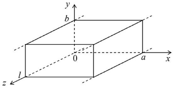 Fig. 7.29. Rectangular metallic-wall resonator as a finite section of a waveguide with the cross-section shown in Fig. 22.
To use the first approach outlined above, let us consider the resonator as a finite-length \ (\Delta \mathrm{z}=l) section of the rectangular waveguide stretched along axis \ z, which was analyzed in detail in Sec. 6. As a reminder, at \ a<b, in the fundamental \ H_{10} traveling wave mode, both vectors E and H do not depend on y, with E having only a y-component. In contrast, H has two components, \ H_{x} and \ H_{z}, with the phase shift \ \pi / 2 between them, and with \ H_{x} having the same phase as \ E_{y} – see Eqs. (131), (137), and (138). Hence, if a plane perpendicular to the z-axis, is placed so that the electric field vanishes on it, \ H_{x} also
vanishes, so that both boundary conditions (104), pertinent to a perfect metallic wall, are fulfilled simultaneously.
As a result, the \ H_{10} wave would not be perturbed by two metallic walls separated by an integer number of half-wavelengths \ \lambda_{z} / 2 corresponding to the wave number given by the combination of Eqs. (102) and (133):
\ k_{z}=\left(k^{2}-k_{t}^{2}\right)^{1 / 2}=\left(\frac{\omega^{2}}{\nu^{2}}-\frac{\pi^{2}}{a^{2}}\right).\tag{7.205}
Using this expression, we see that the smallest of these distances, \ l=\lambda_{\mathrm{z}} / 2=\pi / k_{\mathrm{z}}, gives the resonance frequency82
\ \omega_{101}=\nu\left[\left(\frac{\pi}{a}\right)^{2}+\left(\frac{\pi}{l}\right)^{2}\right]^{1 / 2},\tag{7.206}
where the indices of \ \omega show the numbers of half-waves along each dimension of the system, in the order \ [a, b, l]. This is the lowest (fundamental) eigenfrequency of the resonator (if \ b<a, l).
The field distribution in this mode is close to that in the corresponding waveguide mode \ H_{10} (Fig. 22), with the important difference that the magnetic and electric fields are now shifted by phase \ \pi / 2 both in space and time, just as in the Fabry-Pérot resonator – see Eqs. (195) and (198). Such a time shift allows for a very simple interpretation of the \ H_{101} mode, which is especially adequate for very flat resonators, with \ b<<a, l. At the instant when the electric field reaches its maximum (Fig. 30a), i.e. when the magnetic field vanishes in the whole volume, the surface electric charge of the walls (with the areal density \ \sigma=E_{n} / \varepsilon) is largest, being localized mostly in the middle of the broadest (in Fig. 30, horizontal) faces of the resonator. At the immediate later times, the walls start to recharge via surface currents, whose density \ J is largest in the side walls, and reaches its maximal value in a quarter of the oscillation period \ \mathcal{T}=2 \pi / \omega_{101} – see Fig. 30b.
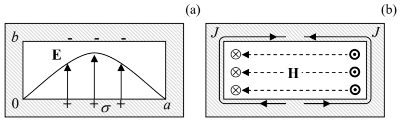
The currents generate the vortex magnetic field, with looped field lines in the plane of the broadest face of the resonator. The surface currents continue to flow in this direction until (in one more quarter period) the broader walls of the resonator are fully recharged in the polarity opposite to that shown in Fig. 30a. After that, the surface currents start to flow in the direction opposite to that shown in Fig. 30b. This process, which repeats again and again, is conceptually similar to the well-known oscillations in a lumped \ LC circuit, with the role of (now, distributed) capacitance played mostly by the broadest faces of the resonator, and that of (now, distributed) inductance, by its narrower walls.
In order to generalize the result (206) to higher oscillation modes, the second of the approaches discussed above is more prudent. Separating the variables in the Helmholtz equation (204) as \ \mathcal{R}(\mathbf{r})=X(x)Y(y)Z(z), we see that \ X, \ Y, and \ Z have to be either sinusoidal or cosinusoidal functions of their arguments, with wave vector components satisfying the characteristic equation
\ k_{x}^{2}+k_{y}^{2}+k_{z}^{2}=k^{2} \equiv \frac{\omega^{2}}{\nu^{2}}\tag{7.207}
In contrast to the wave propagation problem, now we are dealing with standing waves along all three dimensions, and have to satisfy the macroscopic boundary conditions (104) on all sets of parallel walls. It is straightforward to check that these conditions \ \left(E_{\tau}=0, H_{n}=0\right) are fulfilled at the following field component distribution:
\ \begin{array}{ll} E_{x}=E_{1} \cos k_{x} x \sin k_{y} y \sin k_{z} z, & H_{x}=H_{1} \sin k_{x} x \cos k_{y} y \cos k_{z} z, \\ E_{y}=E_{2} \sin k_{x} x \cos k_{y} y \sin k_{z} z, & H_{y}=H_{2} \cos k_{x} x \sin k_{y} y \cos k_{z} z, \\ E_{z}=E_{3} \sin k_{x} x \sin k_{y} y \cos k_{z} z, & H_{z}=H_{3} \cos k_{x} x \cos k_{y} y \sin k_{z} z, \end{array}\tag{7.208}
with each of the wave vector components having an equidistant spectrum, similar to Eq. (196):
\ k_{x}=\frac{\pi n}{a}, \quad k_{y}=\frac{\pi m}{b}, \quad k_{z}=\frac{\pi p}{l},\tag{7.209}
so that the full spectrum of eigenfrequencies is given by the following formula,
\ \omega_{n m p}=\nu k=\nu\left[\left(\frac{\pi n}{a}\right)^{2}+\left(\frac{\pi m}{b}\right)^{2}+\left(\frac{\pi p}{l}\right)^{2}\right]^{1 / 2},\tag{7.210}
which is a natural generalization of Eq. (206). Note, however, that of the three integers \ m, \ n, and \ p, at least two have to be different from zero to keep the fields (208) from vanishing at all points.
We may use Eq. (210), in particular, to evaluate the number of different modes in a relatively small range \ d^{3} k<<k^{3} of the wave vector space, which is, on the other hand, much larger than the reciprocal volume, \ 1 / V=1 / a b l, of the resonator. Taking into account that each eigenfrequency (210), with \ nml \neq 0, corresponds to two field modes with different polarizations,83 the argumentation absolutely similar to the one used for the 2D case at the end of Sec. 7, yields
\ \text{Oscillation mode density}\quad\quad\quad\quad d N=2 V \frac{d^{3} k}{(2 \pi)^{3}}.\tag{7.211}
This property, valid for resonators of arbitrary shape, is broadly used in classical and quantum statistical physics,84 in the following form. If some electromagnetic mode functional \ f(\mathbf{k}) is a smooth function of the wave vector k, and the volume \ V is large enough, then Eq. (211) may be used to approximate the
sum of the functional’s values over the modes by an integral:
\ \sum_{\mathbf{k}} f(\mathbf{k}) \approx \int_{N} f(\mathbf{k}) d N \equiv \int_{\mathbf{k}} f(\mathbf{k}) \frac{d N}{d^{3} k} d^{3} k=2 \frac{V}{(2 \pi)^{3}} \int_{\mathbf{k}} f(\mathbf{k}) d^{3} k.\tag{7.212}
Leaving similar analyses of resonant cavities of other shapes for the reader’s exercise, let me finish this section by noting that low-loss resonators may be also formed by finite length sections of not only metallic-wall waveguides of various cross-sections, but also of the dielectric waveguides. Moreover, even a simple slab of a dielectric material with a \ \mu / \varepsilon ratio substantially different from that of its environment (say, the free space) may be used as a high-Q Fabry-Pérot interferometer (Fig. 31), due to an effective wave reflection from its surfaces at normal and especially inclined incidence – see, respectively, Eqs. (68), and Eqs. (91) and (95).
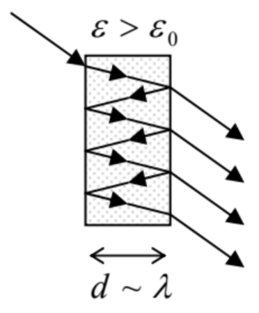 Fig. 7.31. A dielectric Fabry-Pérot interferometer.
Actually, such dielectric Fabry-Pérot interferometers are frequently more convenient for practical purposes than metallic-wall resonators, not only due to possibly lower losses (especially in the optical range), but also due to a natural coupling to the environment, that enables a ready way of wave insertion and extraction – see Fig. 31 again. The backside of the same medal is that this coupling to the environment provides an additional mechanism of power losses, limiting the resonance quality – see the next section.
Reference
79 The device is named after its inventors, Charles Fabry and Alfred Pérot; is also called the Fabry-Pérot etalon (meaning “gauge”), because of its initial usage for the light wavelength measurements.
80 The resonators formed by well conducting (usually, metallic) walls are frequently called resonant cavities.
81 This is of course the expression of the first of the general boundary conditions (104). The second of these conditions (for the magnetic field) is satisfied automatically for the transverse waves we are considering.
82 In most electrical engineering handbooks, the index corresponding to the shortest side of the resonator is listed last, so that the fundamental mode is nominated as \ H_{110} and its eigenfrequency as \ \omega_{110}.
83 This fact becomes evident from plugging Eqs. (208) into the Maxwell equation \ \nabla \cdot \mathbf{E}=0. The resulting equation, \ k_{x} E_{1}+k_{y} E_{2}+k_{z} E_{3}=0, with the discrete, equidistant spectrum (209) for each wave vector component, may be satisfied by two linearly independent sets of the constants \ E_{1,2,3}.
84 See, e.g., QM Sec. 1.1 and SM Sec. 2.6.