6.8: Exercise Problems

6.1. Use Eq. (14) to prove the following general form of the Hellmann-Feynman theorem (whose proof in the wave-mechanics domain was the task of Problem 1.5): \[\frac{\partial E_{n}}{\partial \lambda}=\left\langle n\left|\frac{\partial \hat{H}}{\partial \lambda}\right| n\right\rangle,\] where \(\lambda\) is an arbitrary \(c\)-number parameter.

6.2. Establish a relation between Eq. (16) and the result of the classical theory of weakly anharmonic ("nonlinear") oscillations at negligible damping.

Hint: You may like to use N. Bohr’s reasoning discussed in Problem 1.1.

6.3. A weak, time-independent force \(F\) is exerted on a 1D particle that was placed into a hardwall potential well \[U(x)= \begin{cases}0, & \text { for } 0<x<a \\ +\infty, & \text { otherwise }\end{cases}\] Calculate, sketch, and discuss the \(1^{\text {st }}\)-order perturbation of its ground-state wavefunction.

6.4. A time-independent force \(\mathbf{F}=\mu\left(\mathbf{n}_{x} y+\mathbf{n}_{y} x\right)\), where \(\mu\) is a small constant, is applied to a \(3 \mathrm{D}\) harmonic oscillator of mass \(m\) and frequency \(\omega_{0}\), located at the origin. Calculate, in the first order of the perturbation theory, the effect of the force upon the ground state energy of the oscillator, and its lowest excited energy level. How small should the constant \(\mu\) be for your results to be quantitatively correct?

6.5. A 1D particle of mass \(m\) is localized at a narrow potential well that may be approximated with a delta function: \[U(x)=-w \delta(x), \quad \text { with } w>0 .\] Calculate the change of its ground state energy by an additional weak, time-independent force \(F\), in the first non-vanishing approximation of the perturbation theory. Discuss the limits of validity of this result, taking into account that at \(F \neq 0\), the localized state of the particle is metastable.

6.6. Use the perturbation theory to calculate the eigenvalues of the operator \(\hat{L}^{2}\) in the limit \(|m| \approx l\) \(>>1\), by purely wave-mechanical means.

Hint: Try the following substitution: \(\Theta(\theta)=f(\theta) / \sin ^{1 / 2} \theta\).

6.7. In the lowest non-vanishing order of the perturbation theory, calculate the shift of the ground-state energy of an electrically charged spherical rotator (i.e. a particle of mass \(m\), free to move over a spherical surface of radius \(R\) ) due to a weak, uniform, time-independent electric field \(\mathscr{E}\). 6.8. Use the perturbation theory to evaluate the effect of a time-independent, uniform electric field \(\mathscr{E}\) on the ground state energy \(E_{\mathrm{g}}\) of a hydrogen atom. In particular:

(i) calculate the \(2^{\text {nd }}\)-order shift of \(E_{\mathrm{g}}\), neglecting the extended unperturbed states with \(E>0\), and bring the result to the simplest analytical form you can,

(ii) find the lower and the upper bounds on the shift, and

(iii) discuss the simplest experimental manifestations of this quadratic Stark effect.

6.9. A particle of mass \(m\), with electric charge \(q\), is in its ground \(s\)-state with a given energy \(E_{\mathrm{g}}<\) 0 , being localized by a very short-range, spherically-symmetric potential well. Calculate its static electric polarizability \(\alpha\).

6.10. In some atoms, the charge-screening effect of other electrons on the motion of each of them may be reasonably well approximated by the replacement of the Coulomb potential \((3.190), U=-C / r\), with the so-called Hulthén potential \[U=-\frac{C / a}{\exp \{r / a\}-1} \rightarrow-C \times \begin{cases}1 / r, & \text { for } r<<a, \\ \exp \{-r / a\} / a, & \text { for } a<<r .\end{cases}\] Assuming that the effective screening radius \(a\) is much larger than \(r_{0} \equiv \hbar^{2} / m C\), use the perturbation theory to calculate the energy spectrum of a single particle of mass \(m\), moving in this potential, in the lowest order needed to lift the \(l\)-degeneracy of the levels.

6.11. In the lowest non-vanishing order of the perturbation theory, calculate the correction to energies of the ground state and all lowest excited states of a hydrogen-like atom/ion, due to electron’s penetration into its nucleus, modeling it as a spinless, uniformly charged sphere of radius \(R<<r_{\mathrm{B}} / Z\).

6.12. Prove that the kinetic-relativistic correction operator (48) indeed has only diagonal matrix elements in the basis of unperturbed Bohr atom states (3.200).

6.13. Calculate the lowest-order relativistic correction to the ground-state energy of a \(1 \mathrm{D}\) harmonic oscillator.

6.14. Use the perturbation theory to calculate the contribution to the magnetic susceptibility \(\chi_{\mathrm{m}}\) of a dilute gas, that is due to the orbital motion of a single electron inside each gas particle. Spell out your result for a spherically-symmetric ground state of the electron, and give am estimate of the magnitude of this orbital susceptibility.

6.15. How to calculate the energy level degeneracy lifting, by a time-independent perturbation, in the \(2^{\text {nd }}\) order of the perturbation in \(\hat{H}^{(1)}\), assuming that it is not lifted in the \(1^{\text {st }}\) order? Carry out such calculation for a plane rotator of mass \(m\) and radius \(R\), carrying electric charge \(q\), and placed into a weak, uniform, constant electric field \(\mathscr{E}\).

6.16. \({ }^{*}\) The Hamiltonian of a quantum system is slowly changed in time.

(i) Develop a theory of quantum transitions in the system, and spell out its result in the \(1^{\text {st }}\) order in the speed of the change. (ii) Use the \(1^{\text {st }}\)-order result to calculate the probability that a finite-time pulse of a slowly changing force \(F(t)\) drives a 1D harmonic oscillator, initially in its ground state, into an excited state.

(iii) Compare the last result with the exact one.

6.17. Use the single-particle model to calculate the complex electric permittivity \(\varepsilon(\omega)\) of a dilute gas of similar atoms, due to their induced electric polarization by a weak external ac field, for a field frequency \(\omega\) very close to one of quantum transition frequencies \(\omega_{n n}\). Based on the result, calculate and estimate the absorption cross-section of each atom.

Hint: In the single-particle model, atom’s properties are determined by \(Z\) similar, non-interacting electrons, each moving in a similar static attracting potential, generally different from the Coulomb one, because it is contributed not only by the nucleus, but also by other electrons.

6.18. Use the solution of the previous problem to generalize the expression for the London dispersion force between two atoms (whose calculation in the harmonic-oscillator model was the subject of Problems \(3.16\) and 5.15) to the single-particle model with an arbitrary energy spectrum.

6.19. Use the solution of the previous problem to calculate the potential energy of interaction of two hydrogen atoms, both in their ground state, separated by distance \(r \gg r_{\mathrm{B}}\).

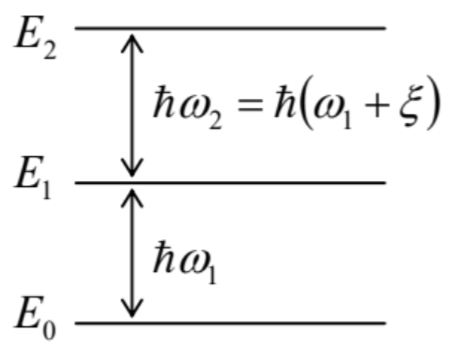
6.20. In a certain quantum system, distances between the three lowest energy levels are slightly different \(-\) see the figure on the right \(\left(|\xi|<<\omega_{1,2}\right)\). Assuming that the involved matrix elements of the perturbation Hamiltonian are known, and are all proportional to the external ac field’s amplitude, find the time necessary to populate the first excited level almost completely (with a given precision \(\varepsilon<<1\) ), using the Rabi oscillation effect, if at \(t=0\) the system is completely in its ground state.

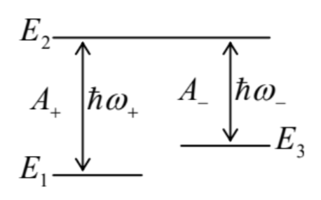
6.21. \({ }^{*}\) Analyze the possibility of a slow transfer of a system from one of its energy levels to another one (in the figure on the right, from level 1 to level \(3)\), using the scheme shown in that figure, in which the monochromatic external excitation amplitudes \(A_{+}\)and \(A_{-}\)may be slowly changed at will.

6.22. A weak external force pulse \(F(t)\), of a finite time duration, is applied to a 1D harmonic oscillator that initially was in its ground state.

(i) Calculate, in the lowest non-vanishing order of the perturbation theory, the probability that the pulse drives the oscillator into its lowest excited state.

(ii) Compare the result with the exact solution of the problem.

(iii) Spell out the perturbative result for a Gaussian-shaped waveform, \[F(t)=F_{0} \exp \left\{-t^{2} / \tau^{2}\right\},\] and analyze its dependence on the scale \(\tau\) of the pulse duration.

6.23. A spatially-uniform, but time-dependent external electric field \(\mathscr{E}(t)\) is applied, starting from \(t=0\), to a charged plane rotator, initially in its ground state. (i) Calculate, in the lowest non-vanishing order in the field’s strength, the probability that by time \(t>0\), the rotator is in its \(n^{\text {th }}\) excited state.

(ii) Spell out and analyze your results for a constant-magnitude field rotating, with a constant angular velocity \(\omega\), within the rotator’s plane.

(iii) Do the same for a monochromatic field of frequency \(\omega\), with a fixed polarization.

6.24. A spin- \(1 / 2\) with a gyromagnetic ratio \(\gamma\) is placed into a magnetic field including a timeindependent component \(\mathscr{B}_{0}\), and a perpendicular field of a constant magnitude \(\mathscr{B}_{\mathrm{r}}\), rotated with a constant angular velocity \(\omega\). Can this magnetic resonance problem be reduced to one already discussed in Chapter 6?

6.25. Develop general theory of quantum excitations of the higher levels of a discrete-spectrum system, initially in the ground state, by a weak time-dependent perturbation, up to the \(2^{\text {nd }}\) order. Spell out and discuss the result for the case of monochromatic excitation, with a nearly perfect tuning of its frequency \(\omega\) to the half of a certain quantum transition frequency \(\omega_{n 0} \equiv\left(E_{n}-E_{0}\right) / \hbar\).

6.26. A heavy, relativistic particle, with electric charge \(q=Z e\), passes by a hydrogen atom, initially in its ground state, with an impact parameter \(b\) within the range \(r_{\mathrm{B}}<<b<<r_{\mathrm{B}} / \alpha\), where \(\alpha \approx\) \(1 / 137\) is the fine structure constant. Calculate the probabilities of the atom’s transition to its lowest excited states.

6.27. A particle of mass \(m\) is initially in the localized ground state, with energy \(E_{\mathrm{g}}<0\), of a very small, spherically-symmetric potential well. Calculate the rate of its delocalization by an applied classical force \(\mathbf{F}(t)=\mathbf{n} F_{0} \cos \omega t\) with a time-independent direction \(\mathbf{n}\).

6.28. \({ }^{*}\) Calculate the rate of ionization of a hydrogen atom, initially in its ground state, by a classical, linearly polarized electromagnetic wave with an electric field’s amplitude \(\mathscr{E}_{0}\), and a frequency \(\omega\) within the range \[\hbar / m_{\mathrm{e}} r_{\mathrm{B}}^{2}<<\omega<c / r_{\mathrm{B}},\] where \(r_{\mathrm{B}}\) is the Bohr radius. Recast your result in terms of the cross-section of electromagnetic wave absorption. Discuss briefly what changes of the theory would be necessary if either of the above conditions had been violated.

6.29. \({ }^{*}\) Use the quantum-mechanical Golden Rule to derive the general expression for the electric current \(I\) through a weak tunnel junction between two conductors, biased with dc voltage \(V\), treating the conductors as degenerate Fermi gases of electrons with negligible direct interaction. Simplify the result in the low-voltage limit.

Hint: The electric current flowing through a weak tunnel junction is so low that it does not substantially perturb the electron states inside each conductor.

6.30 .{ }^{*}\) Generalize the result of the previous problem to the case when a weak tunnel junction is biased with voltage \(V(t)=V_{0}+A \cos \omega t\), with \(\hbar \omega\) generally comparable with \(e V_{0}\) and \(e A\).

6.31 .{ }^{*}\) Use the quantum-mechanical Golden Rule to derive the Landau-Zener formula (2.257).