2.12: Charge Images

So far, we have discussed various methods of solution of the Laplace boundary problem (35). Let us now move on to the discussion of its generalization, the Poisson equation (1.41), that we need when besides conductors, we also have stand-alone charges with a known spatial distribution \(\ \rho(\mathbf{r})\). (This will also allow us, better equipped, to revisit the Laplace problem in the next section.)

Let us start with a somewhat limited, but very useful charge image (or “image charge”) method. Consider a very simple problem: a single point charge near a conducting half-space – see Fig. 26.

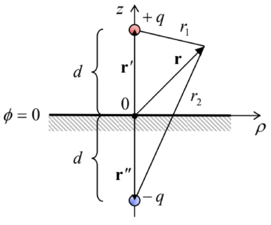Fig. 2.26. The simplest problem readily solvable by the charge image method. The points’ colors are used, as before, to denote the charges of the original (red) and opposite (blue) sign.

Let us prove that its solution, above the conductor’s surface \(\ (z \geq 0)\), may be represented as:

\[\ \phi(\mathbf{r})=\frac{1}{4 \pi \varepsilon_{0}}\left(\frac{q}{r_{1}}-\frac{q}{r_{2}}\right) \equiv \frac{q}{4 \pi \varepsilon_{0}}\left(\frac{1}{\left|\mathbf{r}-\mathbf{r}^{\prime}\right|}-\frac{1}{\left|\mathbf{r}-\mathbf{r}^{\prime \prime}\right|}\right),\tag{2.185}\]

or in a more explicit form, using the cylindrical coordinates shown in Fig. 26:

\[\ \phi(\mathbf{r})=\frac{q}{4 \pi \varepsilon_{0}}\left(\frac{1}{\left[\rho^{2}+(z-d)^{2}\right]^{1 / 2}}-\frac{1}{\left[\rho^{2}+(z+d)^{2}\right]^{1 / 2}}\right),\tag{2.186}\]

where \(\ \rho\) is the distance of the observation point from the “vertical” line on which the charge is located. Indeed, this solution evidently satisfies both the boundary condition \(\ \phi=0\) at the surface of the conductor \(\ (z=0)\), and the Poisson equation (1.41), with the single \(\ \delta\)-functional source at point \(\ \mathbf{r}^{\prime}=\{0,0, d\}\) on its right-hand side, because the second singularity of the solution, at point \(\ \mathbf{r}”=\{0,0,-d\}\), is outside the region of the solution’s validity \(\ (z \geq 0)\). Physically, this solution may be interpreted as the sum of the fields of the actual charge \(\ (+q)\) at point \(\ \mathbf{r}^{\prime}\), and an equal but opposite charge \(\ (-q)\) at the “mirror image” point \(\ \mathbf{r}^{\prime \prime}\) (Fig. 26). This is the basic idea of the charge image method. Before moving on to more complex problems, let us discuss the situation shown in Fig. 26 in a little bit more detail, due to its fundamental importance.

First, we can use Eqs. (3) and (186) to calculate the surface charge density:

\[\ \sigma=-\left.\varepsilon_{0} \frac{\partial \phi}{\partial z}\right|_{z=0}=-\frac{q}{4 \pi} \frac{\partial}{\partial z}\left(\frac{1}{\left[\rho^{2}+(z-d)^{2}\right]^{1 / 2}}-\frac{1}{\left[\rho^{2}+(z+d)^{2}\right]^{1 / 2}}\right)_{z=0}=-\frac{q}{4 \pi} \frac{2 d}{\left(\rho^{2}+d^{2}\right)^{3 / 2}}.\tag{2.187}\]

From this, the total surface charge is

\[\ Q=\int_{S} \sigma d^{2} r=2 \pi \int_{0}^{\infty} \sigma(\rho) \rho d \rho=-\frac{q}{2} \int_{0}^{\infty} \frac{2 d}{\left(\rho^{2}+d^{2}\right)^{3 / 2}} \rho d \rho.\tag{2.188}\]

This integral may be easily worked out using the substitution \(\ \xi \equiv \rho^{2} / d^{2}\) (giving \(\ d \xi=2 \rho d \rho / d^{2}\)):

\[\ Q=-\frac{q}{2} \int_{0}^{\infty} \frac{d \xi}{(\xi+1)^{3 / 2}}=-q\tag{2.189}\]

This result is very natural: the conductor brings as much surface charge from its interior to the surface as necessary to fully compensate the initial charge \(\ (+q)\) and hence to kill the electric field at large distances as efficiently as possible, hence reducing the total electrostatic energy (1.65) to the lowest possible value.

For a better feeling of this polarization charge of the surface, let us take our calculations to the extreme – to the \(\ q\) equal to one elementary change \(\ e\), and place a particle with this charge (for example, a proton) at a macroscopic distance – say 1 m – from the conductor’s surface. Then, according to Eq. (189), the total polarization charge of the surface equals to that of an electron, and according to Eq. (187), its spatial extent is of the order of \(\ d^{2}=1 \mathrm{~m}^{2}\). This means that if we consider a much smaller part of the surface, \(\ \Delta A<<d^{2}\), its polarization charge magnitude \(\ \Delta Q=\sigma \Delta A\) is much less than one electron! For example, Eq. (187) shows that the polarization charge of quite a macroscopic area \(\ \Delta A=1 \mathrm{~cm}^{2}\) right under the initial charge \(\ (\rho=0)\) is \(\ e \Delta A / 2 \pi d^{2} \approx 1.6 \times 10^{-5} e\). Can this be true, or our theory is somehow limited to the charges \(\ q\) much larger than \(\ e\)? (After all, the theory is substantially based on the approximate macroscopic model (1); maybe this is the culprit?)

Surprisingly enough, the answer to this question has become clear (at least to some physicists :-) only as late as in the mid-1980s when several experiments demonstrated, and theorists accepted, some rather grudgingly, that the usual polarization charge formulas are valid for elementary charges as well, i.e., such the polarization charge \(\ \Delta Q\) of a macroscopic surface area can indeed be less than \(\ e\). The underlying reason for this paradox is the physical nature of the polarization charge of a conductor’s surface: as was discussed in Sec. 1, it is due not to new charged particles brought into the conductor (such charge would be in fact quantized in the units of e), but to a small shift of the free charges of a conductor by a very small distance from their equilibrium positions that they had in the absence of the external field induced by charge \(\ q\). This shift is not quantized, at least on the scale relevant to our problem, and hence neither is \(\ \Delta Q\).

This understanding has paved the way toward the invention and experimental demonstration of several new devices including so-called single-electron transistors,⁵⁸ which may be used, in particular, for ultrasensitive measurement of polarization charges as small as \(\ \sim 10^{-6} e\). Another important class of single-electron devices is the dc and ac current standards based on the fundamental relation \(\ I=-ef\), where \(\ I\) is the dc current carried by electrons transferred with the frequency \(\ f\). The experimentally achieved⁵⁹ relative accuracy of such standards is of the order of \(\ 10^{-7}\), and is not too far from that provided by the competing approach based on a combination of the Josephson effect and the quantum Hall effect.⁶⁰

Second, let us find the potential energy \(\ U\) of the charge-to-surface interaction. For that, we may use the value of the electrostatic potential (185) at the point of the charge itself \(\ \left(\mathbf{r}=\mathbf{r}^{\prime}\right)\), of course ignoring the infinite potential created by the real charge, so that the remaining potential is that of the image charge

\[\ \phi_{\text {image }}\left(\mathbf{r}^{\prime}\right)=-\frac{1}{4 \pi \varepsilon_{0}} \frac{q}{2 d}.\tag{2.190}\]

Looking at the electrostatic potential’s definition given by Eq. (1.31), it may be tempting to immediately write \(\ U=q \phi_{\text {image }}=-\left(1 / 4 \pi \varepsilon_{0}\right)\left(q^{2} / 2 d\right)\) [WRONG!], but this would be incorrect. The reason is that the potential \(\ \phi_{\text {image }}\) is not independent of \(\ q\), but is actually induced by this charge. This is why the correct approach is to calculate \(\ U\) from Eq. (1.61), with just one term:

\[\ U=\frac{1}{2} q \phi_{\text {image }}=-\frac{1}{4 \pi \varepsilon_{0}} \frac{q^{2}}{4 d},\tag{2.191}\]

giving twice lower energy than in the wrong result cited above. To double-check Eq. (191), and also get a better feeling of the factor \(\ 1/2\) that distinguishes it from the wrong guess, we can calculate \(\ U\) as the integral of the force exerted on the charge by the conductor’s surface charge (i.e., in our formalism, by the image charge):

\[\ U=-\int_{\infty}^{d} F(z) d z=\frac{1}{4 \pi \varepsilon_{0}} \int_{\infty}^{d} \frac{q^{2}}{(2 z)^{2}} d z=-\frac{1}{4 \pi \varepsilon_{0}} \frac{q^{2}}{4 d}.\tag{2.192}\]

This calculation clearly accounts for the gradual build-up of the force \(\ F\), as the real charge is being brought from afar (where we have opted for \(\ U =0\)) toward the surface.

This result has several important applications. For example, let us plot the electrostatic energy \(\ U\) of an electron, i.e. a particle with charge \(\ q=-e\), near a metallic surface, as a function of \(\ d\). For that, we may use Eq. (191) until our macroscopic model (1) becomes invalid, and \(\ U\) transitions to some negative constant value \(\ (-\psi)\) inside the conductor – see Fig. 27a. Since our calculation was for an electron with zero potential energy at infinity, at relatively low temperatures, \(\ k_{\mathrm{B}} T<<\psi\), electrons in metals may occupy only the states with energies below \(\ -\psi\) (the so-called Fermi level⁶¹). The positive constant \(\ \psi\) is called the workfunction because it describes the smallest work necessary to remove the electron from a metal. As was discussed in Sec. 1, in good metals the electric field screening takes place at interatomic distances \(\ a_{0} \approx 10^{-10} \mathrm{~m}\). Plugging \(\ d=a_{0}\) and \(\ q=-e\) into Eq. (191), we get \(\ \psi \approx 6 \times 10^{-19} \mathrm{~J} \approx 3.5 \mathrm{eV}\). This crude estimate is in surprisingly good agreement with the experimental values of the workfunction, ranging between 4 and 5 eV for most metals.⁶²

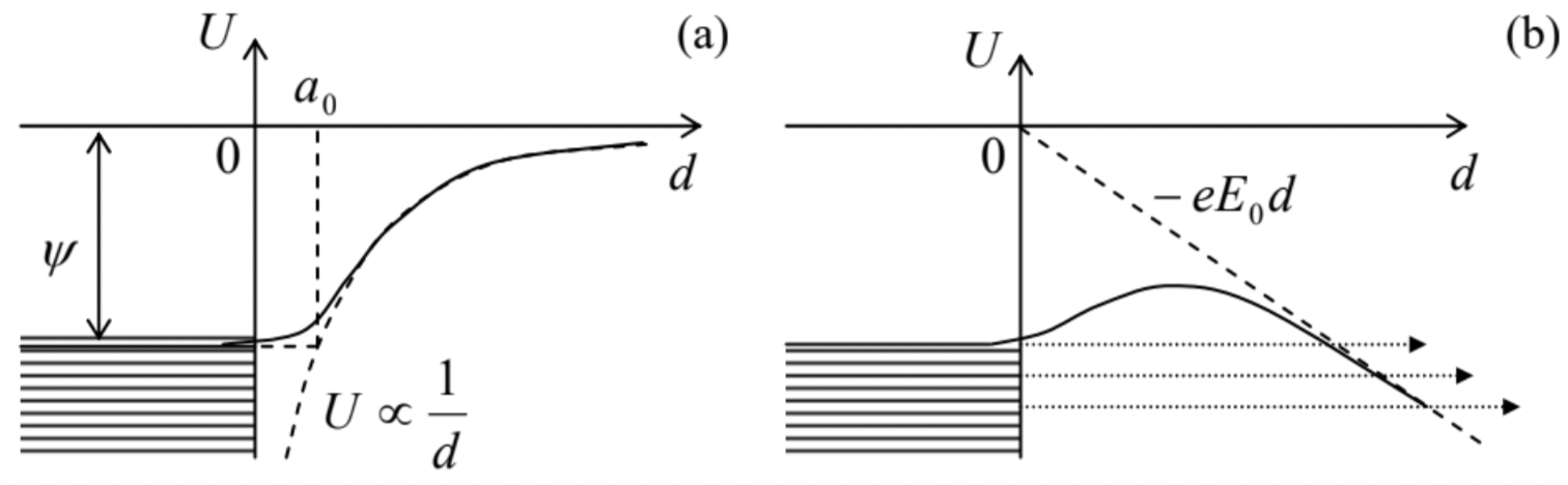Fig. 2.27. (a) The origin of the workfunction, and (b) the field emission of electrons (schematically).

Next, let us consider the effect of an additional uniform external electric field \(\ \mathbf{E}_{0}\) applied normally to a metallic surface, on this potential profile. We can add the potential energy that the field gives to the electron at distance \(\ d\) from the surface, \(\ U_{\mathrm{ext}}=-e E_{0} d\), to that created by the image charge. (As we know from Eq. (1.53), since the field \(\ \mathbf{E}_{0}\) is independent of the electron’s position, its recalculation into the potential energy does not require the coefficient 1⁄2.) As the result, the potential energy of an electron near the surface becomes

\[\ U(d)=-e E_{0} d-\frac{1}{4 \pi \varepsilon_{0}} \frac{e^{2}}{4 d}, \quad \text { for } d>a_{0},\tag{2.193}\]

with a similar crossover to \(\ U=-\psi\) inside the conductor – see Fig. 27b. One can see that at the appropriate sign, and a sufficient magnitude of the applied field, it lowers the potential barrier that prevents electrons from leaving the conductor. At \(\ E_{0} \sim \psi / a_{0}\) (for metals, \(\ \sim 10^{10} \mathrm{~V} / \mathrm{m}\)), this suppression becomes so strong that electrons with energies at, and just below the Fermi level start quantum-mechanical tunneling through the remaining thin barrier. This is the field electron emission (or just “field emission”) effect, which is used in vacuum electronics to provide efficient cathodes that do not require heating to high temperatures.⁶³

Returning to the basic electrostatics, let us find some other conductor geometries where the method of charge images may be effectively applied. First, let us consider a right angle corner (Fig. 28a). Reflecting the initial charge in the vertical plane we get the image shown in the top left corner of that panel. This image makes the boundary condition \(\ \phi=\text { const }\) satisfied on the vertical surface of the corner. However, for the same to be true on the horizontal surface, we have to reflect both the initial charge and the image charge in the horizontal plane, flipping their signs. The final configuration of four charges, shown in Fig. 28a, evidently satisfies all boundary conditions. The resulting potential distribution may be readily written as the generalization of Eq. (185). From it, the electric field and electric charge distributions, and the potential energy and forces acting on the charge may be calculated exactly as above – an easy exercise left for the reader.

Next, consider a corner with angle \(\ \pi / 4\) (Fig. 28b). Here we need to repeat the reflection operation not two but four times before we arrive at the final pattern of eight positive and negative charges. (Any attempt to continue this process would lead to overlap with the already existing charges.) This reasoning may be readily extended to corners of angles \(\ \beta=\pi / n\), with any integer \(\ n\), which require \(\ 2n\) charges (including the initial one) to satisfy all the boundary conditions.

Fig. 2.28. The charge images for (a, b) the corners with angles \(\ \pi\) and \(\ \pi / 2\), (c) a plane capacitor, and (d) a rectangular box; (e) the typical equipotential surfaces for the last system.

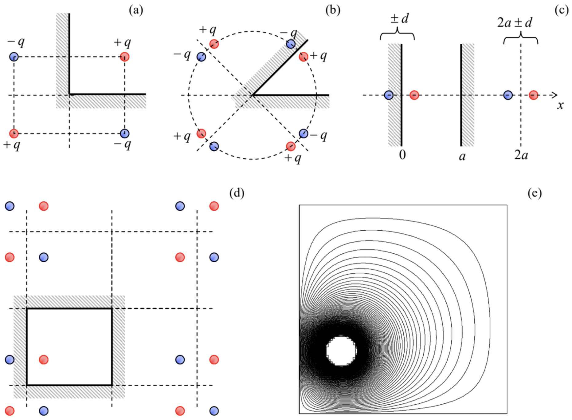
Some configurations require an infinite number of images but are still tractable. The most important of them is a system of two parallel conducting surfaces, i.e. an unbiased plane capacitor of infinite area (Fig. 28c). Here the repeated reflection leads to an infinite system of charges \(\ \pm q\) at points

\[\ x_{j}^{\pm}=2 a j \pm d,\tag{2.194}\]

where \(\ d\) (with \(\ 0<d<a\)) is the position of the initial charge, and \(\ j\) an arbitrary integer. The resulting infinite sum for the potential of the real charge \(\ q\), created by the field of its images,

\[\ \phi(d)=\frac{1}{4 \pi \varepsilon_{0}}\left[-\frac{q}{2 d}+\sum_{j \neq 0} \sum_{\pm} \frac{\pm q}{\left|d-x_{j}^{\pm}\right|}\right] \equiv-\frac{q}{4 \pi \varepsilon_{0}}\left\{\frac{1}{2 d}+\frac{d^{2}}{a^{3}} \sum_{j=1}^{\infty} \frac{1}{j\left[j^{2}-(d / a)^{2}\right]}\right\},\tag{2.195}\]

is converging (in its last form) very fast. For example, the exact value, \(\ \phi(a / 2)=-2 \ln 2\left(q / 4 \pi \varepsilon_{0} a\right)\), differs by less than 5% from the approximation using just the first term of the sum.

The same method may be applied to 2D (cylindrical) and 3D rectangular conducting boxes that require, respectively, 2D or 3D infinite rectangular lattices of images; for example in a 3D box with sides \(\ a\), \(\ b\), and \(\ c\), charges \(\ \pm q\) are located at points (Fig. 28d)

\[\ \mathbf{r}_{j k l}^{\pm}=2 j a+2 k b+2 l c \pm \mathbf{r}^{\prime}\tag{2.196}\]

where \(\ \mathbf{r’}\) is the location of the initial (real) charge, and \(\ j\), \(\ k\), and \(\ l\) are arbitrary integers. Figure 28e shows a typical result of the summation of the potentials of such charge set, including the real one, in a 2D box (within the plane of the real charge). One can see that the equipotential surfaces, concentric near the charge, are naturally leaning along the conducting walls of the box, which have to be equipotential.

Even more surprisingly, the image charge method works very efficiently not only for rectilinear geometries, but also for spherical ones. Indeed, let us consider a point charge \(\ q\) at distance \(\ d\) from the center of a conducting, grounded sphere of radius R (Fig. 29a), and try to satisfy the boundary condition \(\ \phi=0\) for the electrostatic potential on the sphere’s surface using an imaginary charge \(\ q^{\prime}\) located at some point beyond the surface, i.e. inside the sphere.

Fig. 2.29. Method of charge images for a conducting sphere: (a) the idea, and (b) the resulting potential distribution in the central plane containing the charge, for the particular case \(\ d=2 R\).

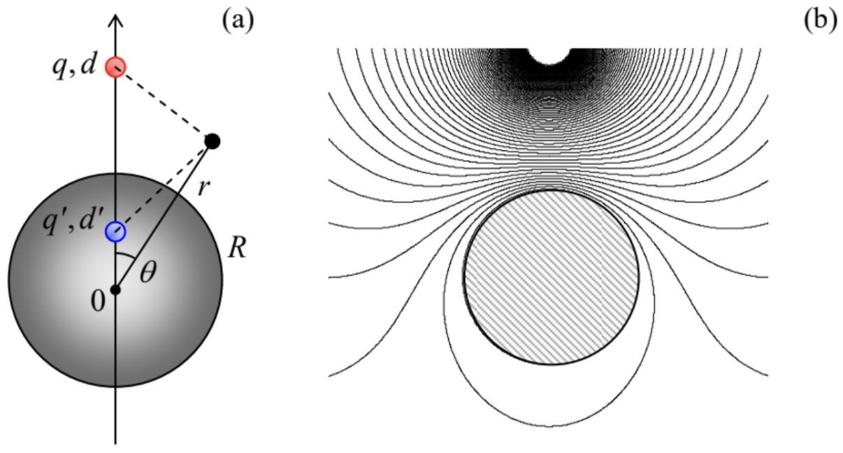
From the problem’s symmetry, it is clear that the point should be at the line passing through the real charge and the sphere’s center, at some distance \(\ d^{\prime}\) from the center. Then the total potential created by the two charges at an arbitrary point with \(\ r \geq R\) (Fig. 29a) is

\[\ \phi(r, \theta)=\frac{1}{4 \pi \varepsilon_{0}}\left[\frac{q}{\left(r^{2}+d^{2}-2 r d \cos \theta\right)^{1 / 2}}+\frac{q^{\prime}}{\left(r^{2}+d^{\prime 2}-2 r d^{\prime} \cos \theta\right)^{1 / 2}}\right].\tag{2.197}\]

This expression shows that we can make the two fractions to be equal and opposite at all points on the sphere’s surface (i.e. for any \(\ \theta\) at \(\ r=R\)), if we take⁶⁴

\[\ d^{\prime}=\frac{R^{2}}{d}, \quad q^{\prime}=-\frac{R}{d} q.\tag{2.198}\]

Since the solution to any Poisson boundary problem is unique, Eqs. (197) and (198) give us the final solution for this problem. Fig. 29b shows a typical equipotential pattern following from this solution. It may be surprising how formulas that simple may describe such an elaborate field distribution.

Now we can calculate the total charge \(\ Q\) on the grounded sphere’s surface, induced by the external charge \(\ q\). We could do this, as we have done for the conducting plane, by the brute-force integration of the surface charge density \(\ \sigma=-\varepsilon_{0} \partial \phi /\left.\partial r\right|_{r=R}\). It is more elegant, however, to use the following Gauss law argument. Equality (197) is valid (at \(\ r \geq R\)) regardless of whether we are dealing with our real problem (charge \(\ q\) and the conducting sphere) or with the equivalent charge configuration – with the point charges \(\ q\) and \(\ q^{\prime}\), but no sphere at all. Hence, according to Eq. (1.16), the Gaussian
integral over a surface with radius \(\ r=R+0\), and the total charge inside the sphere should be also the same. Hence we immediately get

\[\ Q=q^{\prime}=-\frac{R}{d} q.\tag{2.199}\]

A similar argumentation may be used to calculate the charge-to-sphere interaction force:

\[\ F=q E_{\text {image }}(d)=q \frac{q^{\prime}}{4 \pi \varepsilon_{0}\left(d-d^{\prime}\right)^{2}}=-\frac{q^{2}}{4 \pi \varepsilon_{0}} \frac{R}{d} \frac{1}{\left(d-R^{2} / d\right)^{2}}=-\frac{q^{2}}{4 \pi \varepsilon_{0}} \frac{R d}{\left(d^{2}-R^{2}\right)^{2}}.\tag{2.200}\]

(Note that this expression is legitimate only at \(\ d>R\).) At large distances, \(\ d >> R\), this attractive force decreases as \(\ 1 / d^{3}\). This unusual dependence arises because, as Eq. (199) specifies, the induced charge of the sphere, responsible for the force, is not constant but decreases as \(\ 1 / d\). In the next chapter, we will see
that such force is also typical for the interaction between a point charge and a point dipole.

All previous formulas were for a sphere that is grounded to keep its potential equal to zero. But what if we keep the sphere galvanically insulated, so that its net charge is fixed, for example, equals zero? Instead of solving this problem from scratch, let us use (again!) the almighty linear superposition principle. For that, we may add to the previous problem an additional charge, equal to \(\ -Q=-q \text {'}\), to the sphere, and argue that this addition gives, at all points, an additional, spherically-symmetric potential that does not depend on the potential induced by the external charge \(\ q\), and was calculated in Sec. 1.2 – see Eq. (1.19). For the interaction force, such addition yields

\[\ F=\frac{q q^{\prime}}{4 \pi \varepsilon_{0}\left(d-d^{\prime}\right)^{2}}+\frac{q q^{\prime}}{4 \pi \varepsilon_{0} d^{2}}=-\frac{q^{2}}{4 \pi \varepsilon_{0}}\left[\frac{R d}{\left(d^{2}-R^{2}\right)^{2}}-\frac{R}{d^{3}}\right].\tag{2.201}\]

At large distances, the two terms proportional to \(\ 1 / d^{3}\) cancel each other, giving \(\ F \propto 1 / d^{5}\). Such a rapid force decay is due to the fact that the field of the uncharged sphere is equivalent to that of two (equal and opposite) induced charges \(\ +q^{\prime}\) and \(\ -q^{\prime}\), and the distance between them (\(\ d-d^{\prime}=d-R^{2} / d\)) tends to zero at \(\ d \rightarrow \infty\). The potential energy of such interaction behaves as \(\ U \propto 1 / d^{6}\) at \(\ d \rightarrow \infty\); in the next chapter we will see that this is the general law of the induced dipole interaction.

---

Reference

⁵⁸ Actually, this term (for which the author of these notes may be blamed :-) is misleading: the operation of the “single-electron transistor” is based on the interplay of discrete charges (multiples of e) transferred between conductors, and sub-single-electron polarization charges – see, e.g., K. Likharev, Proc. IEEE 87, 606 (1999).

⁵⁹ See, e.g., M. Keller et al., Appl. Phys. Lett. 69, 1804 (1996) ; F. Stein et al., Metrologia 54, 1 (2017).

⁶⁰ J. Brun-Pickard et al., Phys. Rev. X 6, 041051 (2016).

⁶¹ More discussion of these states may be found in SM Secs. 3.3 and 6.3.

⁶² More discussion of the workfunction, and its effect on the electrons’ kinetics, is given in SM Sec. 6.3.

⁶³ The practical use of such “cold” cathodes is affected by the fact that, as it follows from our discussion in Sec. 4, any nanoscale irregularity of a conducting surface (a protrusion, an atomic cluster, or even a single “adatom” stuck to it) may cause a strong increase of the local field well above the applied uniform field \(\ E_{0}\), making the electron emission reproducibility and stability in time significant challenges. In addition, the impact-ionization effects may lead to an avalanche-type electric breakdown already at fields as low as \(\ \sim 3 \times 10^{6} \mathrm{~V} / \mathrm{m}\).

⁶⁴ In geometry, such points with \(\ d d^{\prime}=R^{2}\), are referred to as the result of mutual inversion in a sphere of radius \(\ R\).